DESIGN & TESTING


Our objective was to build a pet robot that integrates computer vision and speech recognition to closely resemble various characteristics of a real pet. Figure 1 displays a high level overview of the project design. The robot uses a microphone to take as input a user's voice commands. This input is passed to a speech recognition engine within the Raspberry Pi which processes and deciphers the voice commands. Once the speech is understood, the Raspbery Pi executes the function corresponding to that voice command. When the command demands that the robot navigate to an object, the OpenCV library is used to enable the robot to autonomously travel towards the ball.

In recognizing speech, the Raspberry Pi searches through the user's command to find key words. If a key word is found, the robot translates the user's voice input to a command that it supports. The list of supported commands is shown in Figure 2. For example, one of the primary commands is the move command, which will move the robot in the specified direction. Other commands, such as saying "hello", will require the robot to reply to the user. For these situations, the robot is programmed with a set of replies that uses speech synthesis to convert strings into voice. The modular design allowed us to work in parallel and minimize dependencies between separate systems. This allowed for a efficient and effective workflow.

final project overview
Phrase Result
Play ball Goes to blue target and then to green target
Forward Moves robot forward
Backward Moves robot backward
Left Turns 90 degrees left and goes straight
Right Turns 90 degrees right and goes straight
Play song Plays a hardcoded song
Hi Replies hello to the user
Figure 1: Overview of Design
Figure 2: Supported commands

SPEECH RECOGNITION


Our initial goal was to use a local speech recognition engine on the Pi so that users can use the speech feature even without access to the Internet. However after testing with the local speech recognition engine, we decided to move to an on-line approach because the engine had a long delay in understanding simple phrases. In the end we used the Google Speech Recognition API to decipher user input. Through our testing, we found that it would take 32 seconds to recognize a pharse locally on the Raspberry Pi, while it would only take 0.04 seconds to recognize the same phrase using the Google Speech Recognition API. Our objective was to make a friendly pet robot that would instantly react to user inputs so we decided to use Google's Speech Recognition API to yield faster responses from the pet.

The local speech recognition was performed by using PocketSphinx. We installed the SpeechRecognition library for Python which easily connects to multiple speech recognition softwares, one of which is the CMU Sphinx engine. The initial setup of Sphinx took much longer than expected. There were many errors with dependencies and incorrect files in the Pi. However after we had gotten it to properly install on the Pi, it was fairly straightforward to get the engine working in a Python script. The functions were simple and there were many examples on how to use the Sphinx engine, and this helped us immensely. The readings were not very accurate but it was able to detect key words which is what we needed. We only spoke short phrases of two to four words so the engine could make a more accurate prediction. We found that longer phrases tended to be more inaccurate. Our major concern with Sphinx was the delay in the recognition. When we said "play ball", it took the engine 34 seconds to understand the phrase. This was not very helpful for our application as we needed the robot to respond quickly to user input. We then looked into other methods for speech recognition which might reduce the delay and allow the robot to work in real-time.

One of the other tools supported by the SpeechRecognition library on Python was the Google Speech Recognition API. One of the main reasons we chose this was that it did not require a special API key unlike the other tools supported by this library. It was as simple as ensuring the dependencies were satisfied and calling the appropriate function. We discovered that the Google Speech Recognition engine was much faster and more reliable than Sphinx. Although this required the Raspberry Pi to be connected to the Internet during speech recognition, the results it gave were perfect for our application. It took the Google Speech Recognition 0.04 seconds to not only decipher the phrase "play ball" but also to go through the servers and reply back to us. Because of the high level of accuracy and tremendously small delay in recognition, we decided to use the Google Speech Recognition instead of Sphinx. We noticed that there were instances when Google would not be able to clearly understand what we were saying. It might have been due to both having a poor quality microphone and the algorithm for recognition itself. In order to increase our chances for detecting keywords, we tried different phrases until it detected a phrase consistently which would have our keyword. For example, it was able to understand the phrase "play fetch" in the beginning. However, it was inconsistent so we decided to change the phrase to "play ball". The new phrase was consistently understood by the recognition engine thereby resulting in better accuracy for this command, which instructed the robot to search search for a blue object and navigate towards it until it reaches it, and then search for a green object and navigate towards it until it reaches it.


SPEECH SYNTHESIS


An important part of the project was to make sure that the robot could reply to users, or ensure we could perform speech synthesis. Instead of making dynamic replies, we decided to make a more basic reply method. When the robot detects an input, it will reply to the user using pre-determined sentences. For example when the user says "Hi", the robot will reply with "Hello". We used the eSpeak library to accomplish speech synthesis. The library would take in strings and would speak them out through the speakers attached to the Raspberry Pi. We decided to go with the default version of voice. It sounded a bit robotic, but it was clear and understandable to the users. Although we implemented this, we were unable to present it during the final demo because our speakers had run out of power. However, the code still works properly so we kept it for this report. We discovered that just using the eSpeak library on Python would give a buffer overflow, so we decided to use the subprocess Python library to execute the commands on the terminal. When eSpeak received the commands on the terminal, it was able to say all of the sentences without causing a buffer overflow. We tested it with both small and large sentences and the eSpeak library was able to say them perfectly.


OVERALL SPEECH SYSTEM


The first step of the speech system was to take in user input through a microphone. At first, we had hoped to leverage the microphone capability of the SpeechRecognition Python library to allow us to handle both the microphone and the speech recognition using just one library. However, we were unable to get the microphone working using the SpeechRecognition library. We then decided to use a different library called PyAudio, which is actually a dependency of the SpeechRecognition library. Using both the PyAudio and Wave libraries, we were able to take user input via a microphone. We used the libraries to gather user input into a wav file. The wav file was stored in the same directory as the main Python file. Every time a user spoke into the microphone, the wav file would be rewritten with the latest user input. We decided this design such that a user was requied to press a button on the the Raspberry Pi before they could give a voice command, allowing the Raspberry Pi to only take user inputs at certain periods of time. This turned out to work much better than listening to the user input at all times which would require a very large amount of compututations. We discuss alternatives to this in the results section. After the user presses the button, the Pi listens for user input for three seconds. Our application supports only small phrases so we decided that 3 seconds was a suitable amount of time. It was enough time for speaker to say the phrases without rushing and short enough to be usable.

The input is then saved as a wav file. The wav file is read by the speech recognition library and sent to Google Speech Recognition engine to understand the user input. The result would then be a string returned from Google of what it thinks the user said. We then search this string for key words. If one of the keywords is present, then the program will perform the command associated with that keyword. Even if many key words are present, our program will only perform the first command that it finds. Some commands will make the robot move while other commands will make the robot reply to the user. In the end, we have a fully functioning robot which, just like a pet, can interpret speech into a set of commands for which it executes the appropriate function, whether it be to move forward, navigate towards an object, or reply in voice.


IMAGE RECOGNITION


We used the OpenCV library to enable the robot to autonomously move towards objects of different color. OpenCV is an open source computer vision software library that interfaces with Python and is focused on real-time applications, making it a great fit for our project. It’s extensive library allowed us to accurately detect different colored objects with very little error. We downloaded OpenCV using this command:

$ sudo apt-get install Python-opencv

Professor Skovira provided us with a Pi Camera, and we chose to use it to equip our robot with vision. The Pi Camera has a very helpful library for obtaining video streams that can be converted to OpenCV objects. We could then manipulate those objects to achieve object detection. Before we could write an application using OpenCV, we had to setup our PiCamera such that it would interface with the computer vision library. This took some time, as it required us to downgrade the PiCamera to version 1.10. The version that the PiCamera came packaged with did not work properly with OpenCV for unknown reasons. However, we were able to set up the PiCamera using the following commands:

$ pip install "picamera[array]"
$ sudo pip install picamera==1.10

We wrote a “Hello World” program to confirm that OpenCV and PiCamera were functioning properly. This program simply accessed the camera and displayed its video stream on the screen. It used the Pi Camera library to create a camera object and used it’s capture_continuous method to return a frame from the video stream. We displayed this frame and verified that there was minimal lag in it’s display. This provided us with a strong foundation towards detecting objects of different color. Our first step was to convert the BGR image obtained from the Pi Camera frame to HSV. We do this because it is easier to represent a color in HSV than it is in the RGB color-space, according to the OpenCV-Python Tutorials. We were looking to locate blue and green objects, so we defined lower and upper threshold values in HSV for these two colors. We obtained these thresholds from the OpenCV-Python Tutorial as well and they are shown in the table below:

Color Lower Upper
Blue (110, 50, 50) (130, 255, 255)
Green (29, 86, 6) (64, 255, 255)
Figure 3: Threshold Values

We create a mask using the OpenCV’s inRange method, which thresholds the HSV image and obtains only colors that fall in the defined range. We then use the erode and dilate methods to remove any noise that may be left in the mask. The findContours function computes the outline of the object. We consider only the largest contour. We made this decision knowing that it would work because we restrained our robot’s environment to a hallway that had very little blue or green colors. We then find the radius of this contour and set a threshold that the radius must exceed for the contour to be considered a valid object. We verified that we were able to accurately detect blue and green objects by simply waving them across the Pi Camera’s vision and printing values when the Pi Camera detected them. We also printed the x-coordinate of the object on the screen to ensure that our program was able to not only detect the object’s presence but also identify its location. This piece of information was integral in navigating our robot towards the object, as is described in the next section.


ROBOT NAVIGATION


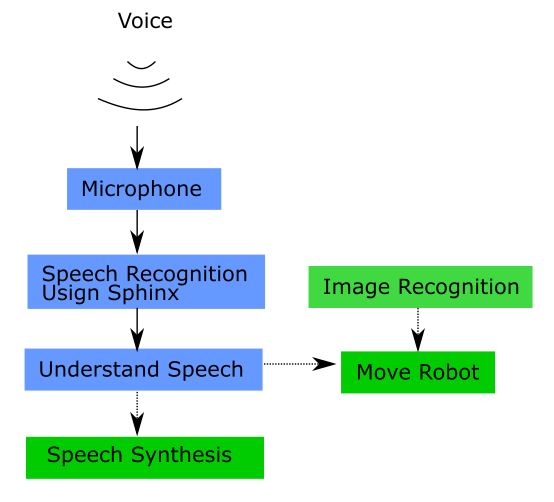
The robot constantly uses information provided by the Pi Camera and OpenCV library to navigate itself towards a green or blue object when prompted. During the navigation, there are four states: Polling, Moving Towards Object, Move Until Lost, and Done. We describe each state below.

Polling

The robot begins in polling state. It looks for the object for 1.3 milliseconds. If it finds a valid object, then it moves into the Moving Towards Object state. If it does not, then the robot turns 30 degrees, and continues looking for the object in the Polling state. This function enabled the robot to find objects even if they were placed behind it, since the robot would eventually make a full 360 degree turn in looking for it. We chose to turn the robot by 30 degree increments so as to not miss any objects but also to keep the navigation efficient. We tested turning the robot by 45 degree increments, but this modification caused the robot to miss object when it was further away from it.

Moving Towards Object

In the moveToTarget() method, the robot first calls the findBall() method which searches for the object. If the object is no longer in the robot’s view, then the findBall() method returns 1000 and causes the robot to move back to the Polling state.

If the object is in the robot’s view and returns a very large radius of over 175, then we deduce that the object is very close to the robot. We determined this assumption through experimentation. In testing our image detection, we also noticed that the Pi Camera would often lose objects that were too close to it. When an object encapsulated the entire camera’s vision, the camera often was not able to detect its color. What led us to look into this matter was our observation that the robot would often navigate perfectly towards the object but then simply pass by it. Hence, we realized that the Pi Camera was unreliable when the robot was about two to three feet away from the object, and we introduced the Move Until Lost state for this reason. When the findBall() method detects an object of a radius of over 175, the robot moves to the Move Until Lost state, and this addition solved the issue of the robot moving past the object after navigating towards it in a seemingly perfect manner. At the Moving Towards Object state, the distance sensor may also cause the robot to move into the Move Until Lost state by detecting the object and therefore signaling that the robot is approximately a foot and a half away from it.

If the findBall() method does not return 900 or 1000, then it returns the x-coordinate of the object. Our window was set to a width of 640 pixels, so the x-coordinate had to be between 0 and 640. We defined three sections within this window and used them to determine which direction to move the robot. If the x-coordinate was less than 160, then the object was to the left of the robot so the robot veered left. If the x-coordinate was greater than 480, then the object was to the right of the robot so the robot veered right. Otherwise, the x-coordinate was between 160 and 480 and thus the object was relatively straight ahead of the robot. In this case, the robot moves straight forward. We did not use any scientific formulas to define these three sections. Rather, we based it off of intuition that as long as the object was in the middle half of the Pi Camera’s vision, the robot should continue to move straight ahead, and this worked very well in keeping the robot on track towards the object.

Move Until Lost

In this state, the robot knows that it is within two to three feet of the object. This state’s objective is to keep the robot moving towards the object until the Pi Camera no longer detects the object or the distance sensor indicates that the robot is within a foot and a half of the object. This conservative approach ensures that the robot will not miss the object and move past it. It does, however, mean that our robot does not go directly up to and touch the object but rather stops about a foot and a half away from it.

The robot will continue to move towards the object in the same exact fashion as it does in the Moving Towards Object state until the Pi Camera ceases to detect the object or the distance sensor detects an object in front of it. When either of those two events occur, the robot moves to the Done state.

Done

The robot is located within a foot and a half of the object. It stops and blinks an LED for 5 seconds. If it is currently at the blue object, then it moves back to the Polling State with the objective of finding the green object. Otherwise, if it is at the green object, it simply waits for its next command.

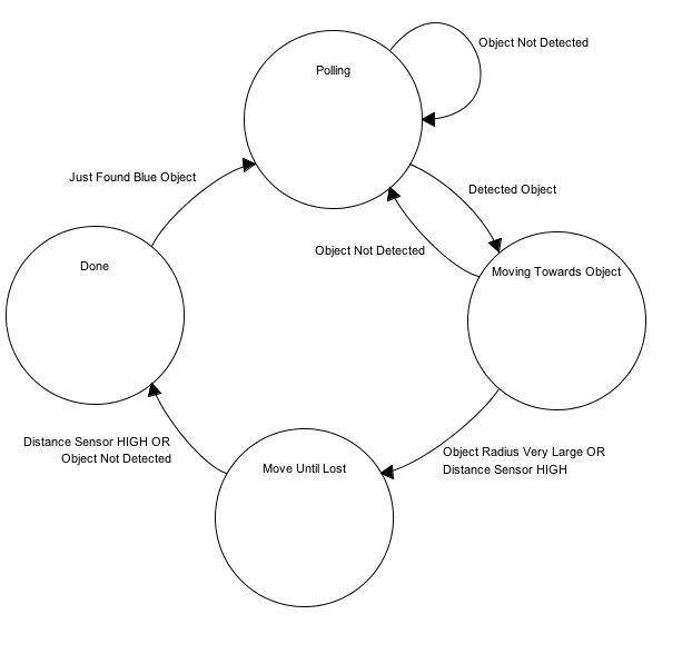
This state machine is shown in the diagram below:

Robot Navigation Finite State Machine
Figure 4: Robot Navigation Finite State Machine


Servos

We used the rpi.GPIO library to control the servos. We chose this library primarily because we had already experimented with this library in a previous lab assignment, so we felt comfortable with its functionalities and uses. It also proved to be sufficient for the task of transporting the robot towards an object. However, the robot did not move as smoothly or as quickly as we may have liked and we concede that an alternative library such as pi-GPIO may have yielded more optimal results. Although we did do our research and looked into using different GPIO libraries, we decided that, given our time constraint, we needed to prioritize detecting the object and navigating our robot towards it before we began to optimize the process.

Using the rpi.GPIO library, we created two PWM instances using the GPIO.PWM(channel, frequency) method, one for each servo. We set the frequency equal to 50 Hz and set the channel equal to the pin number corresponding to the servo. We found that a duty cycle of approximately 6.3 resulted in the fastest clockwise direction and that a duty cycle of approximately 7.8 resulted in the fasted counterclockwise direction. We used this information to write helper methods that move the robot forward and backward and turn the robot right or left.

Copyright © , Judy Stephen and Cameron Boroumand

Using theme by BlackTie.co