Pointybot
Kristina nemeth (Kan57) and Cuyler Crandall (csc254) WEdnesday Lab
Introduction
PointyBot was developed by Kristina Nemeth and Cuyler Crandall, working remotely from Florida and Ithaca, respectively. The hardware for PointyBot includes a dual-axis pointed driven by a pair of servos in conjunction with two absolute value encoders, alongside a GPS and IMU which provide sensing to determine the system’s position and orientation. The system runs on a Raspberry Pi 3 and users interact with it via touchscreen commands on a PiTFT display. In software, PointyBot executes two code loops in parallel: a foreground one which users interact with that constantly updates the position of the module and of its targets, and a background loop which ensures that the pointer is constantly oriented towards the module’s target.
AUV.jpg)
Objective
PointyBot is a system which provides a physical representation of the direction another specified point is relative to PointyBot. Though baselined for a static use case tracking a distant target—the International Space Station in orbit—the fundamentals of PointyBot’s operation can be generalized into a number of other applications. Such applications include, but are not limited to: a heads-up display for navigation, an antenna tracking array for remote controlled drones, or a reminder system to indicate where your phone was last placed. Our implementation of the PointyBot included ISS tracking and the ability to point to a number of different preprogrammed locations. The user of PointyBot could choose between these different options using a GUI.

Pointer Design and Testing
Hardware Selection
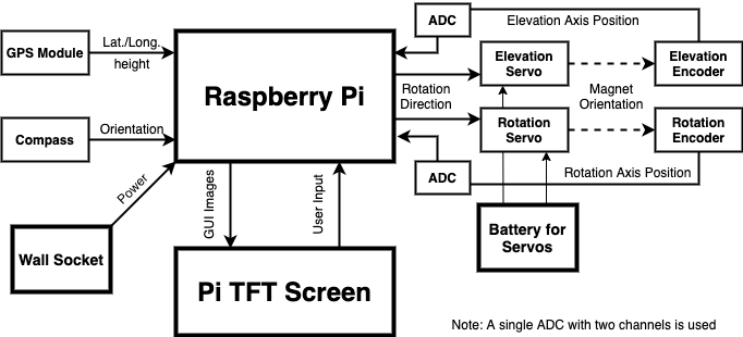
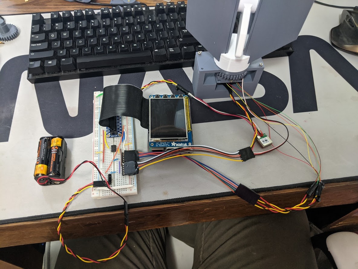
One of the first steps in our project was to determine what hardware was required for us to meet our desired functionality criteria, while remaining under budget with some space in case there were unexpected additional expenses later in the project. Some aspects of the hardware were immediately determined as necessary based on the objectives at hand. Two servos were necessary to move the pointer in the rotation and elevation axes. We decided to use the two servos that were given to us and used in Lab 3 because they were already available, and we had previously used them successfully. To determine the exact positioning of the servos and send the data back to the Raspberry Pi, encoders were necessary. We selected the AS5600 encoders because of their low price and ability to provide data over PWM. We then determined that a slip ring was necessary to support the connection to both servos and encoders with the movement of the robot in the different directions without wires being tangled. In order for PointyBot to know what direction to point in, data about its position regarding orientation and overall location. To determine location, a GPS module was the obvious solution. However, we were severely limited by the price range, which led us to select the GP-20U7 since it was the least expensive option. We decided to use a magnetometer to get the heading information and selected the MPU-9250 based on its price and the ability to communicate to it over I2C. Additionally, this IMU had a python library available for easy integration. Additionally, we wanted to use the TFT to provide user input to the system. After initial testing of the encoders, we determined ADC’s were also necessary for the conversion of the PWM value. We selected the MCP3002 because it was a low cost two channel ADC that could easily communicate data to the Raspberry Pi over SPI. To power the system, we used a battery pack for the servos and a wall socket connection for the Raspberry Pi. A separate battery back is necessary for the servo’s because the current draw of them is too high for the Raspberry Pi pins to support, and also the servo’s introduce a large amount of noise into the system. The entire hardware system follows the diagram shown below. A breadboard was used for all of the immediate connections to the GPS, IMU, and ADC’s. Beyond this header connectors were used for the connectors to the encoders and the servo’s. All of the wiring connects were very straightforward and were almost always direct connections. The only exception to this were resistors that were used on the GPIO lines to protect the pins.
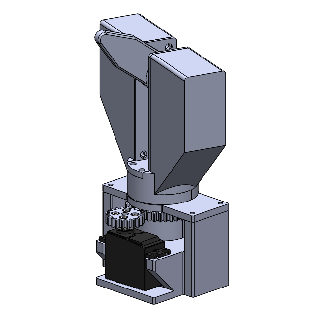
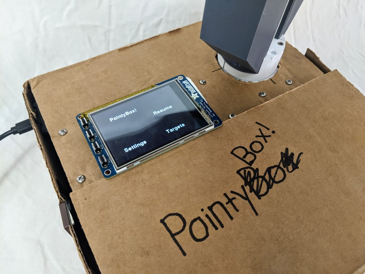
To create the pointing mechanism, we used Solidworks to create a CAD. Following this, we used a 3D printer to build out the components. Two iterations of the CAD were printed before reaching the final form. The 3D printer stopped working before we were able to make a base for the robot, so we used the box our ADCs arrived in.
Encoder Testing
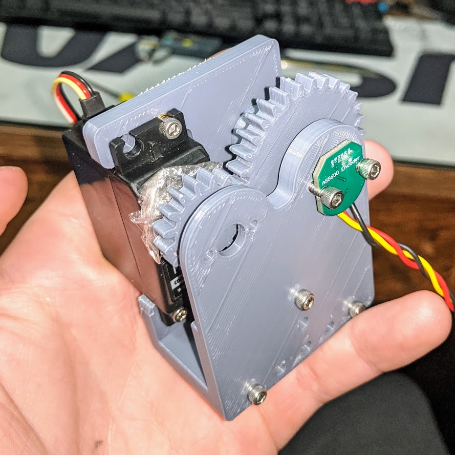
One of the first steps in designing the output was to design and print a simple test rig to test reading the output of our encoders and controlling the position of an axis using a servo. The test rig, pictured below, successfully provided us with information about what needed to be changed for the project to work, namely the need for better servo horns and and ADC, since we could not accurately read the PWM output of the encoder using the Pi alone. Because of these revealed shortcomings of our current setup, the test rig was never fully implemented as the delay between ordering and receiving the required components was long enough for the full dual-axis pointer to be designed and printed. The encoder test rig, as well as all other custom parts for the project, were printed on a Prusa i3 Mk3S and assembled with #4-40 hardware and heat-set inserts.
Designing the Pointer
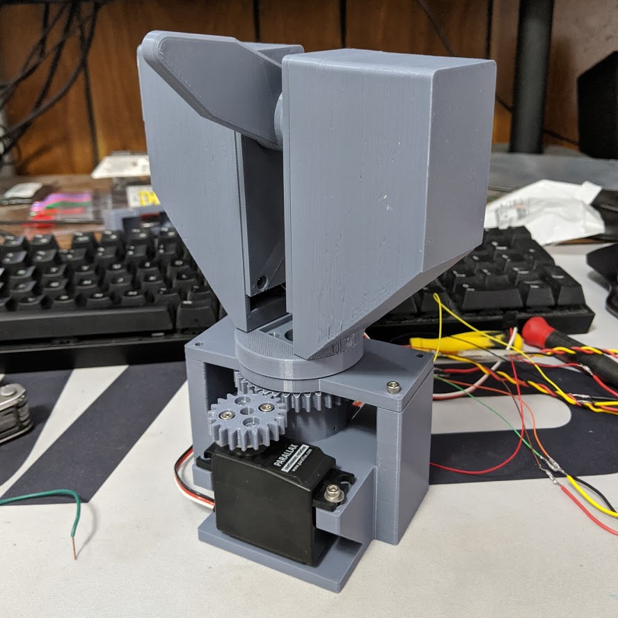
Next came designing and printing the dual-axis pointing mechanism which out system controls. Two majors goals for the pointer were to have no rotational constraints, as well as to be able to directly read the orientation of each axis (as opposed only keeping track of a relative position and recalibrating each power cycle). To accomplish this, the rotation axis of the pointer includes a hollow slip ring which all wires for the elevation axis servo and encoder pass through. Due to this design all of the wires are cordoned off to either rotating or non-rotating sections of the pointer, and the pointer has no rotational limitations, visible below in the image of the rotation stage on its own (wires for the elevation servo coming out the top). Like the encoder test rig the pointer was printed on a Pursa Mk3. The initial batch of parts was printed in grey, with later white parts added to finish out the design and replace elements which were not properly toleranced during the first batch of prints.
Setting Up the ADC
To set up the ADC, we placed it on the breadboard hooked up the corresponding pins to the SPI pins for SPI, PWR, and GND following the datasheet in Reference 4. We decided to power the ADC at 5V since the sampling frequency correlates to the voltage, and we wanted to have the highest possible sampling rate. Initially, we connected the ADC to SPI0 in order to confirm overall functionality. We set up SPI based on the instructions in Reference 2. However, when we tried to confirm the overall functionality of SPI we did not see the correct system response upon entering the command “ls /dev/*spi*”. After some debugging, we realized that this SPI system was already being used by the TFT. Since we initially prioritized the functionality of the ADC over the TFT, we removed the TFT and connected the ADC channel. This decision allowed us to make sure that the ADC and SPI would be fully functional before trying to set up the secondary SPI channel. Additionally, if we ran into errors when setting up SPI1 we would be able to know if the errors were because of the SPI channel and not the ADC. To disable the TFT input, it was necessary to comment out the line “dtoverlay=pitft28-resistive,rotate=90,speed=64000000,fps=30” in “/boot/config.txt”. Follow this, we were able to see the SPI channel. We then wrote a baseline ADC code that would read data from both channels. This code was based off of the code found in Reference [9]. However, at this point we were still not reading data properly. After probing a large amount of signals, we saw that the voltage levels when probing power and ground on the ADC were not corresponding to the desired values. We removed the ADC to rewire it and saw that the breadboard had been melted. This high temperature was consistent with incorrect wiring or a short that connected power to ground, so we determined that this ADC had been blown up. We traced back the cause of this to incorrect wiring connection from breakout connector from the ADC. Luckily we had an extra ADC and wired this up. At this point, we were able to read data from both of the SPI channels. We compared the data that was being read to the data that we saw when probing with a multimeter to confirm functionality. Because our desired application was to read in the average of different PWM data, we set up a list that would save a certain amount of data for PWM channels and then average this over an amount of time to have a voltage. We modified the time over which this was averaged and compared the output values until we determined that they were accurate. We then decided to switch this functionality to SPI1. We re-commented the line to enable the TFT and then followed the steps described in the later section “How to Use SPI1”. We were able to connect the ADC over SPI1 and get the same accurate data readings. To confirm the accuracy of the channel readings over SPI1, we once again probed with a multimeter and compared this with the data readings from the multimeter.
Defining the Axes in Code
In code the axes were represented using an axis object which included an encoder and servo object within them. By structuring their code representation in this way, it was easy to tweak the axes without needing to worry about rigid pin assignments or orientations that might change over time. A major component of the axes was figuring out how to properly calibrate them, which was eventually done in two steps: calibrating the mapping of encoder readings on each axis, then determining what direction the axis moved in relation to its servo. The mapping of encoder voltage to axis position was accomplished by prompting the user to move the axis to 0 degrees, then 90, 180, and 270, taking a voltage reading of the encoder at each location. These readings could then be used to determine the roughly linear relationship between angle and encoder voltage in slope-intercept form, the inverse of which would be used to translate later readings to angles. Since this calibration would remain (theoretically) accurate until the pointer was disassembled for some reason, it was stored as a text file, and were that file deleted a user would be prompted to go through the calibration process again the next time an axis was initialized in code. Initially this calibration technique was successful but after a few days two issues were noticed: that one axis was completely incorrect and unable to find specified directions after being reassembled and another was slightly off in its readings (~0-20 degrees scaled at different points). The axis which was seemingly non-functional turned out to be a software issue, though the calibration procedure took in four data points (at 0, 90, 180, and 270 degrees), only 0 and 90 were used to calculate the slope of the degree to voltage conversion. As such, if the 0 to 3.3V cutoff was between 0 and 90 degrees the slope and associated conversion factor were useless. Changing from a single slope to the median value of the 4 slopes between reasons resolved this issue permanently. The cause of the slight error on the other axis was significantly more difficult to tease out of the system, and would have been nearly impossible had we not had access to a multimeter to probe parts of our breadboard. When plugged in, our GPS’ additional current draw caused a 0.5V dip in our 3.3V supply voltage on the rail opposite where the RPi’s 3.3V pin was connected (which our encoders and GPS were attached to). So, if the readings were calibrated without the GPS plugged in and then it were plugged in, each angle mapped to 0 to 0.5V less than previously. The issue was thankfully resolved by adding extra wires between the 3.3V lines as well as re-calibrating any time components were un- or re-plugged into the system. With those bugs resolved we had a system which could point at specified angles relatively accurately. Another function built into the axes code is pulsing the servo and taking readings a series of times when the axis is initialized to determine what orientation the axis is calibrated to relative to the servo. Though this could have been included in the manual calibration process detailed above, it also served as visual feedback of the state of the pointer when powered on, as during later in the project high variability in the servos’ performance was observed.
Determining Pointing Direction
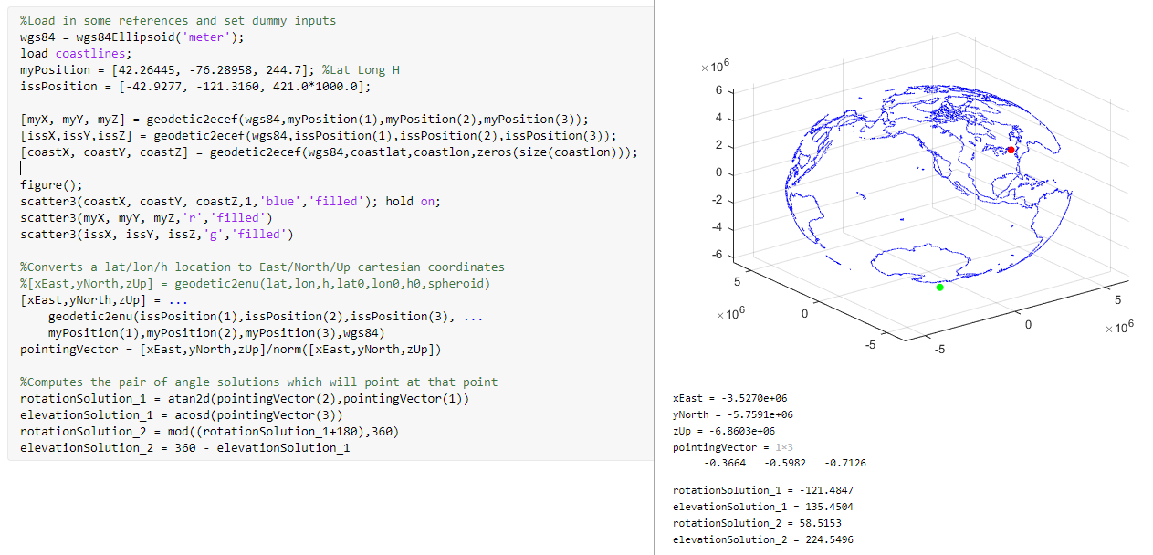
Now that the axes could point towards any set of angles, a system to convert a given position/orientation of PointyBot and location of a target into pointer angles was required. For this math we initially turned to Matlab, since built-in functionality there for coordinate conversions and plotting coastlines makes visualizing what direction a pair of locations should be outputting easier. The key function to all of the math is geodetic2enu, which takes in an origin (in the form of longitude, latitude, and height) as well as a target in the same format, and returns the location of the target in East/North/Up (enu) coordinates. Such a function is incredibly powerful for our uses because it bridges the gap between the geodetic coordinates that the module and target locations are reported in and the cartesian coordinates that we can apply vector math and traditional coordinate transforms to. With the enu pointing vector determined, a bit more math is required to translate it to a pair of angles about the rotation and elevation axes of the module, ensuring that both valid solutions are found and considered. Finally, an offset is applied to the rotation solutions to account for the angular difference between the module’s orientation and due East. With this pipeline for transferring a module location and target into required angles developed in Matlab, it had to be rewritten in Python to run on the Pi. The vector math was available in numpy, but geodetic2enu required tracking down a Python package called pymap3d [6] which emulated functionality of the matlab function. Once written the outputs in python were checked against Matlab to ensure that they were consistent. On the Pi the scripts pull latitude, longitude, height, and orientation of the module and its target from two separate files, updating whenever the contents of those files change. Once the two possible orientations are computed, the script also checks the current orientation of the pointer and selects the closer orientation solution as the new target.
Smoothing Out Issues
With the entire pipeline for converting a position and target into pointing in a desired direction worked out, a great deal of time was dedicated to improving the functionality of this side of the system. During this time a high degree of variability in the servos’ ability to move the pointer’s two axes was noticed, and initially was attributed to run down batteries and/or increased friction in the system during different reassemblies of the axes. Over time it became clear that something was fundamentally wrong about how the servos were being implemented. A number of solutions were attempted, including but not limited to replacing batteries numerous times, editing 3D printed parts to reduce friction losses which could stall the servos, switching from software to hardware PWM (using pigpio [7]), moving what folder the code was run out of, and running the servos sequentially as opposed to simultaneously. All of these changes resulted in the axes working as expected sometimes, but none of them resulted in the axes working as expected at all times. Testing with an Arduino verified that the servos themselves were indeed capable of moving the axes, but without an oscilloscope we were not able to see the output signals being sent to the servos to determine what exactly the issue could be. In the end these issues were not fully resolved, but a configuration was found that allowed the pointer to consistently work, just never as well as intended.
Input Data and Other Code Design and Testing
Magnetometer Data
A modular approach was taken to setting up the Magnetometer sensor data. First, we worked on setting up the sensor data working on its own prior to implementing it within the entire code block. After wiring the sensor up, the first step was to enable I2C on the Raspberry Pi. We followed the guide found in Reference 2. To make sure that it was properly enabled, we ran the command “ls /dev/*i2c*” and got the desired output of “/dev/i2c-l”. A testing code block of data was set up using the MPU-9250 library found in Reference 1 which would read the input values from the accelerometer and print them to the command line. This baseline code was based on the example code found in Reference 1. To confirm the functionality of the sensor, we moved the sensor around and saw if the values changed in a way that corresponded properly to the movement. The next step in this implementation was to derive a header value from the given sensor data. First, we needed to calibrate our sensor. We set up the calibration modeling the steps found in Reference 3. We took thirty seconds worth of data with the sensor moving around and modified the maximum and minimum values according to the data values. Following this we found, the offset to be the sum of the minimum and max values divided by two and then the scaling to be the difference between the two values divided by two. To confirm that this was working properly we saved all of the data into a text file for reference. The next step was to determine how these values correlated to heading. We rotated the IMU to each of the cardinal directions and gathered data. Following this we plotted the data and found a best fit equation for the relationship between each of the points on a scale of 0 to 360 using MATLAB. We then used these equations to derive the angle. However, at this point we started to run into issues because the heading values did not properly correlate to the angle of the sensor. Follow this we gathered more data that was both scaled and unscaled and found that the sensor data only followed the same best fit line at the same position. The data supporting this along with the best fit line can be seen below in Figure X. At this point after conversations with Professor Skovira, we realized that magnetometers would not universally work indoors, and the sensor could only be calibrated to one specific location. We ended up using the best fit line which correlated to the raw sensor data since this functioned well for a single position. In the end, we were able to get heading if the Pointybot did not change locations. We hardcoded in a value for the Pointybot to be pointing north for all of the situations that were not located at the single calibration point.

GPS Data
A similar modular approach to setting up the magnetometer data was used when setting up the GPS data. Initially, an individual interface to the GPS was set up to confirm that data gathering was possible. First, serial was set up on the Raspberry Pi to enable UART using the steps described in Reference 11. Following this, “ls -l /dev” was run to confirm that the mapping for serial connections was properly done. The GPS used can be found in Reference 12. This GPS connection was slightly janky because there was only a transmit pin connection available from the module. The GPS was powered by 3.3V and was connected to the corresponding pins on the RPi. Following this, a baseline code to pull data from the GPS was set up based on the code found in Reference 11. At this point, we were able to read data from the module. We used the website found in Reference 8 to confirm that the location information was correct. This GPS delivered the data in several forms, however the data form we used was GPGGA. The next step was to get the data from the GPS into a usable form. Since the data was continuously being transmitted, it could not be controlled. We decided to save all the data that was being read for 15 seconds into a text file. Follow this, we would process the data. GPGGA data was the only kind of GPS data that had two G’s in a row. The data from the text file was read and saved into a list, and the list was iterated through to find the location where there were two consecutive G characters. From this point, the characters that correspond to the latitude, longitude, height, and corresponding direction were saved. This data then needed to be converted from degree, arc minute, and arc second values to decimal degrees. To complete this conversion, the arc minute values were divided by 60, and the arc second values were divided by 3600. Then the three values were added together. Additionally, the latitude and longitude data needed to be converted to negative if their cardinal direction was South or West. At this point, the GPS data was in the necessary form for it to be properly processed. This data was then written to a file titled moduleInfo.py so that the process in charge of pointing in a specific direction could use it.
ISS Data
In order to properly track the ISS, we needed to consistently be able to pull information about the location of the ISS. To do this we used an API that pulls the ISS location found in Reference 5. Using this we were able to get the latitude and longitude of the ISS. Our code for this was based on the code found in Reference 5. To confirm this data, we compared the values that were displayed once we pulled data with the current location of an ISS. Since both the ISS moves relatively slowly and the PointyBot moves slowly, the position data does not need to be consistently polled for tracking to be completed well. For this reason, a timer was set up to pull data every 5 seconds and then to update the target location based on this. Threading was used to set this timer up and call the function that would gather ISS data again.
Integration
The next stage of working on the inputs was to confirm the integrated functionality of gathering data. To do this, each of the data gathering peripherals (ADC, Magnetometer, and GPS) were run while all three of them were enabled. The IMU immediately worked while all of the other connections were enabled. However, when SPI was enabled UART would no longer function. To debug this, we disabled all the other external connections to see if the UART communication would work. When it was the only thing running, UART was functional again. We then slowly started to set up each of the peripherals again. At this point, UART continued to run again while all of the peripherals were added. This allowed us to confirm that there was no interference between UART and other components. While we are not exactly sure what caused this issue, our best guess is that there was potentially a brownout issue that led to one of the components to function in a weird state.
TFT Interface
To allow for a user to easily interface and control the PointyBot, we used a TFT with a GUI. Other options that could have been implemented would be an application or a website to interface with this. However, the GUI on the TFT was the best option based on the time. The GUI was divided into three main screens: the home screen, settings, and target screen. The target screen was the most important one because this is what allowed the user to choose between ISS tracking, pointing at the ECE 5725 lab, or pointing at a house. To set up the TFT interface the pygame library was used. For easy integration into the main project, we created a separate python file with helper functions that correlated to the display of each of the individual screens.
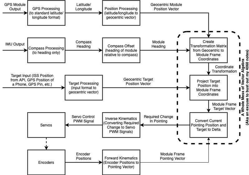
Overall Code Flow
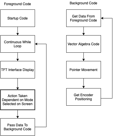
Once all of the individual module aspects were completed, all of the code needed to be integrated together in a functional way. At the start of the project, we determined that the data between all of the modules should flow together based on the diagram shown below in the block diagram. We then decided that the best way to implement this code organization was to create two parallel running processes: a foreground process that would run the GUI on the TFT, gather all of the necessary data, and determine the task that the PointyBot would be taking and a background process that would be responsible for control of the servos and getting the PointyBot to point at a given direction. The interactions within both of these processes can be seen in the block diagram below. The data that needed to be shared between the foreground and background was position data for the robot which included the latitude, longitude, height, and heading data. This data was shared through a separate moduleInfo.py. The foreground code was set up on startup to gather data about the position of the robot and then to display the GUI. Due to the issue with the magnetometer, only the GPS data gathering code was set up to run within the main function. Based on the user input, the user could then set the PointyBot to track the ISS or to point to the preprogrammed locations of ECE5725 Lab, Cuyler’s House or Kristina’s House. The supporting code necessary to implement the tasks commanded in the foreground were turned into helper functions for smooth integration into the final product. The background process followed the steps described by the pointer functionality. We then wrote a bash script to call the foreground and background processes to run together. Following this, we tested the system together. To test, we iterated through the commands and checked to see the direction that the PointyBot was pointing to and checked the data that was being written to the saved files on the Raspberry Pi. One problem that we ran into while testing the robot all together was that the threading timer for gathering position data for the ISS would continue to be called even after ISS tracking was terminated and the PointyBot was set to point at a target location. To fix this, we added another variable to this setup that would only allow the ISS tracking to continue when it was externally called. Other issues with troubleshooting and testing the system together were minor glitches that included the incorrect order of data being written and the incorrect calling order of helper functions.
How To SPI1
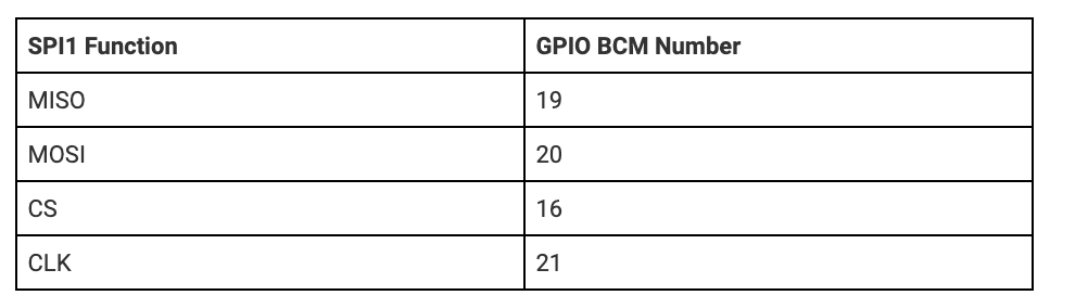
The first steps of setting up SPI1 are the same as setting up SPI0. The first thing was installing the spidev package with the command “pip install spidev”. Following this, SPI needed to be enabled on the Raspberry Pi in raspi-config following the steps detailed in Reference 2. Following this, the /boot/config.txt needs to be modified to include the line “dtoverlay=spi1-3cs” as described in Reference 10. At this point, the Raspberry Pi needs to be rebooted. Following this, the command “ls /dev/*spi*” needs to be run. The desired output response should be “dev/spidev1.0 dev/spidev1.1 and dev/spidev1.2”. 1.0 corresponds to SPI bus 1 device 0 and incrementing accordingly. The SPI connection needs to be wired up, and the pins corresponding to the SPI1 channel are shown below. The wiring should not be done in a 1:1 way, but rather it should be done so that it corresponds to the data flow. For example, the master out slave in pin on the RPi should correspond to the Data in pin on the SPI device. Following this, the device can be interfaced with. However, the code needs to be properly set up to interface with SPI1 instead of SPI 0. When calling the line, spi.open(bus, device) the correct bus and device needs to be selected. When we were setting this up, the only functional device was number 2. We are not exactly sure why this is the case, but it may be helpful to iterate through the device numbers when debugging.
Results
PointyBot—or rather, PointyBox—achieves almost all of the functionality included in our baseline. With the exception of being able to accurately determine its heading, PointyBot is able to determine its position and then dynamically track the relative direction of the ISS, functionality demonstrated in a sped-up timelapse in our project video. Additionally, it is able to point several predetermined GPS locations. It is able to properly interface to all of the external hardware including the GPS, magnetometer, ADC, encoders, and servos. A custom 3D printed pointer was designed to facilitate this functionality. The physical limitations of the output side of the system and associated optimization for slow but accurate tracking means that its useful functionality is largely limited to this baseline.
Conclusion
As mentioned above, the end result of our project was a PointyBot that kind of worked, not as we’d hoped but far from non-functional. Along the way, however, we did discover a number of things which contributed to our limited success… as well as a number of areas which thoroughly hampered progress. A successful area of the project, both from a functional and project management standpoint was the decision to have the input foreground and output background halves of our code communicate via writing to or reading from files of variables. Using this structure the halves of the code could be written largely independently of each other, since the output could be tested by simply writing and saving the appropriate files, and the input could be tested by ensuring that it was outputting files of the correct format. It also allowed for a large degree of flexibility in terms of increasing or decreasing the amount of information being passed around, since increasing the number of variables in the files had no impact on what the output was trying to read from them (as opposed to having to update function calls and parameters if the two were more closely linked). In terms of things which conclusively didn’t work, a majority of these were tied to the input side of the project, not because output was devoid of issues, but because many of its issues did not have conclusive resolutions. For example, our numerous issues with getting the servos to properly turn the output axes were indicative that something was wrong in how we commanded them (especially because the servos were perfectly capable when driven off of an Arduino), but on our Pi there was no consistency between running them with software PWM vs hardware PWM, simultaneously vs sequentially, or even what folder the code was run in. Had we had access to an oscilloscope then we might have more conclusive answers to them in terms of what caused things to not work, but as it stands we do not. On the other hand, in our input system we have a much better idea of what went wrong: don’t expect a magnetometer to work indoors.
Future Work
With more time and a larger budget for the project, two areas are immediately identifiable within the project: determining the orientation of the unit and the output’s ability to track axes in motion. Replacing PointyBot’s IMU with a more robust magnetometer that is capable of getting accurate geodetic heading readings while inside a building (such as the Adafruit BNO055) would solve the former issue with minimal impact on the rest of the system or its code, though it would push the system out of the project’s $100 budget. Fixing the output is a significantly larger challenge, and the interconnectedness of the physical system and how code should be structured to control it means that improving tracking would equate to redesigning the entire output, both physically and digitally. As discussed above, the output’s current structure is centered around the fact that the minimum constant rotation rate of the axes is greater than the maximum accurate tracking speed of the encoders. From a mechanical standpoint, this can be addressed by the addition of bearings and a larger gear reduction between motors and axes to the effect of reducing the power required to overcome friction, as well as lowering maximum tracking rate overall. In addition to this, electrical filtering on the encoder signals would likely help smooth out the jumps in readings which threw off the system previously. With these physical changes in place, the code would have to be restructured to provide constant motion to the axes, as opposed to the intermittent stepping of the current design. Completing these changes would bring PointyBot from its current state to one more closely aligned with our initial vision for the project, but was beyond the time, manufacturing, and budgetary limitations of the past 6 weeks. Given the abundance of Covid-related extra time we will have in the near future, it is likely that we will pursue these changes and develop a cleaner v2 of the system.
References
Reference [1]: https://github.com/FaBoPlatform/FaBo9AXIS-MPU9250-Python
Reference [2]: https://learn.sparkfun.com/tutorials/raspberry-pi-spi-and-i2c-tutorial/all Reference [3]: https://github.com/kriswiner/MPU6050/wiki/Simple-and-Effective-Magnetometer-Calibration
Reference [4]: http://ww1.microchip.com/downloads/en/DeviceDoc/21294E.pdf
Reference [5]: http://open-notify.org/Open-Notify-API/ISS-Location-Now/
Reference [6]: https://pypi.org/project/pymap3d/
Reference [7]: http://abyz.me.uk/rpi/pigpio/python.html#hardware_PWM
Reference [8]: https://www.latlong.net/
Reference [10]: https://tutorials.technology/tutorials/69-Enable-additonal-spi-ports-on-the-raspberrypi.html
Reference [11]: https://www.electronicwings.com/raspberry-pi/raspberry-pi-uart-communication-using-python-and-c
Reference [12]: https://cdn.sparkfun.com/datasheets/GPS/GP-20U7.pdf
Lab manuals 1-3 of ECE 5725 (Spring 2020) were also referenced in the pre-project setup of our Raspberry Pi.
Memeber
Cuyler
Worked on the physical side of PointyBot since the hardware remained with him in Ithaca. Handled the mechanical design, assembly, and testing of the pointer, as well as the background processes which ran it.
Kristina
Worked on setting up, writing code, and testing all of the peripherals and data gathering hardware including the Accelerometer, GPS, and the ADC’s. Virtually helped with the wiring of the electrical system.
Both
Worked on the video, wrote the report, wrote the foreground code process, and debugged the system.
Bill of Materials
| Part | Supplier | Qty. | Total Cost |
|---|---|---|---|
| Raspberry Pi 3 | ECE 5725 | 1 | n/a |
| PiTFT Touchscreen | ECE 5725 | 1 | n/a |
| Parallax Servo | ECE 5725 | 2 | n/a |
| Solderless Breadboard | ECE 5725 | 1 | n/a |
| 5v RPi Power Supply | ECE 5725 | 1 | n/a |
| 6v AA Battery Pack | ECE 5725 | 1 | n/a |
| Assorted resistors and wires | ECE 5725 | ? | n/a |
| AS5600 Absolute Value Encoders | Amazon | 2 | $19.98 |
| Taidacent Hollow Slip Ring (6 Wire) | Amazon | 1 | $20.75 |
| Metal Servo Horns | Amazon | 2 | $2.80 |
| GPS Receiver - GP-20U7 (56 Channel) | Sparkfun | 1 | $17.95 |
| SparkFun IMU Breakout - MPU-9250 | Sparkfun | 1 | $14.95 |
| MCP3002-I/P ADC | Digikey | 1 | $1.79 |
| Cardboard Shipping Box | Digikey | 1 | $0.00 |
| Panel Mount Micro USB Extender | Amazon | 1 | $6.99 |
| Neodymium Magnet (⅛” Thick, ¼” OD) | McMaster | 2 | $2.92 |
| #4-40 SHCS, 5/16” Length | McMaster | ? | ~$1.00 |
| #4-40 Pan Head Screws, 5/16” Length | McMaster | 4 | $0.20 |
| #4-40 Heat Set Inserts | McMaster | ? | ~$2.00 |
| PLA Filament | Amazon | ? | ~$4.00 |
| $95.33 |
![]()
![]()
![]()
![]()