Fun with Irrigation!
Jackson Kopitz jsk363
Peter Cook pac256
May 15, 2019
Objective
In this project, our objective was to build a tree irrigation system that measures and irrigates an amount of water calculated using data from the weather forecast and tree water pressure, in order to maintain constant ideal water pressure in the tree’s transport system.
Introduction
To complete the water irrigation system, we worked with students in the chemical engineering graduate program. These students had been working on the irrigation model and were testing it using a specific set of weather/pressure data. The main directive we were concerned with was properly measuring and irrigating the correct amount of water as reported by the algorithm they had implemented. To do this, we used a Raspberry Pi, a solenoid valve, a flow meter, a bucket, plastic tubing, and waterproofing materials (silicone caulk and epoxy).
Design and Testing
Week 1
We began to meet with Corentin Bisot and Rui Gao in the chemical engineering department to discuss what we would be doing over the last month of the semester. When we first met, we discussed the irrigation algorithm they had originally implemented and what was necessary to make it successfully irrigate proper amounts of water to the tree to maintain an ideal constant water potential. Their code [8] takes in weather data from forecasts and water potential data from a IoT-based data logger in the field, and uses it to iteratively compute the solution to an ordinary differential equation using Euler’s method, in the form of an irrigation rate for the duration of the next time step (dt in the differential equation). This system is modeled as an RC circuit, with dependent sources and parameters determined by the data from external sources, depicted below.
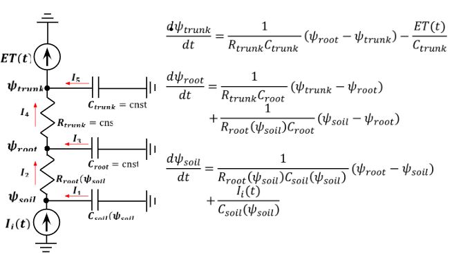
Figure 1: Water potential in tree, modeled as an RC circuit with dependent sources [1]
We planned both to implement the physical device that irrigated the desired amount of water and to fetch the weather and water potential data on our raspberry pi from the internet and IoT platforms, respectively. Furthermore, we talked about the necessary capabilities of our physical system: it needed to be able to release between 1cL and 5L over the course of 1 hour, with granularity of 1cL or less. We thus had a general idea for this first step- we would use GPIO interrupts and a valve to irrigate amounts of water determined by algorithm. The algorithm returned an irrigation rate u1 in kg/s, so in a given time interval we needed to irrigate dt*u1/p liters of water, where p = 1kg/1L, the density of water at STP.
We also started to test parts individually as our friends in the chemical engineering department had a 12V solenoid valve and a relay to switch the valve on and off using GPIO pins on the raspberry pi. For this application, the relay is necessary since the raspberry pi cannot provide large enough voltage or sink enough current to operate the valve. There was some concern operating the valve because it consistently got very hot when powered for a nontrivial period of time, but inspecting the specifications [2], we found that its operating range capped at 80C (very hot) and that we could step down the voltage while maintaining proper operation. When we changed the DC voltage supply to about 7V, 1.86A, it heated up quite a bit less. We also developed a python script to control the relay with a simple GPIO.output to the pin we connected it to called valve.py. Unfortunately, this did not work when we ran some initial tests, and we spent quite a bit of time in the next week getting the relay to work as expected.
Week 2
This week we finalized our system design. The main decision that we made was to decide how to measure the amount of water needed to be irrigated. One option was to use drip irrigation. With this method, the water leaves the irrigator at a slow and constant rate. Thus, we could experimentally find the rate at which the water leaves the irrigator, connect the irrigator to the solenoid valve, and then keep the valve open as long as the irrigator needed to irrigate the given amount of water. The second option was to use a flowmeter to measure the given amount of water. With this option, we could open the valve to allow water flow and then close the valve once the flowmeter measured the given amount of water. The water could then leave the valve and flowmeter to the tree. We chose the latter option. Because the valve opens when it is connected to power, the second option would use much less power because it is only open for the small time it takes for the given amount of water to flow through the valve and irrigator. Assuming the amount to irrigate is between 350mL and 3.5L and that we found water to flow at about 60mL/s experimentally, the second method only require the valve to be open from about 5.8 to 58 seconds. The first option could require the valve to be open for nearly the entire irrigation period (up to 60 minutes).
After choosing a way to measure the amount of water to irrigate, we were able to design the mechanical components of the system. We decided that the water source of our system would be a hose, which would connect to the valve via a ¾” to ½” pipe adapter. The valve would then connect to the flowmeter which would release water into a bucket. The bucket would then either be tilted or have a component inside to get all water to flow to one hole. This hole would be connected to a tube to get the water to where it needed to go. Additionally, since our process of watering the tree needs to be started reliably at the same time every day and we will likely not have access to ethernet/wifi in the field, we decided we needed a real time clock to keep track of time. Below is a sketch of our system design.
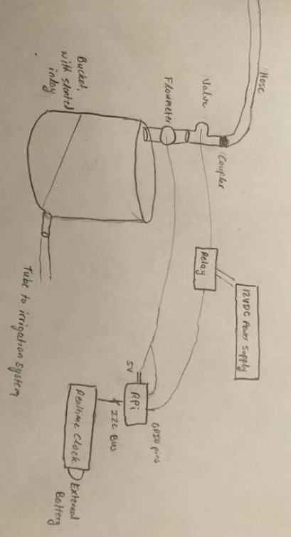
Figure 2: Sketch of initial system design
After we accepted this system design, we needed to buy the required materials. We first went to Lowe’s hardware store to buy the necessary materials we did not have yet- a bucket, tubing, pipe converters, silicone caulk, and epoxy. Next, we purchased the flowmeter and a real time clock module from adafruit. Below are images of our parts pre assembly.
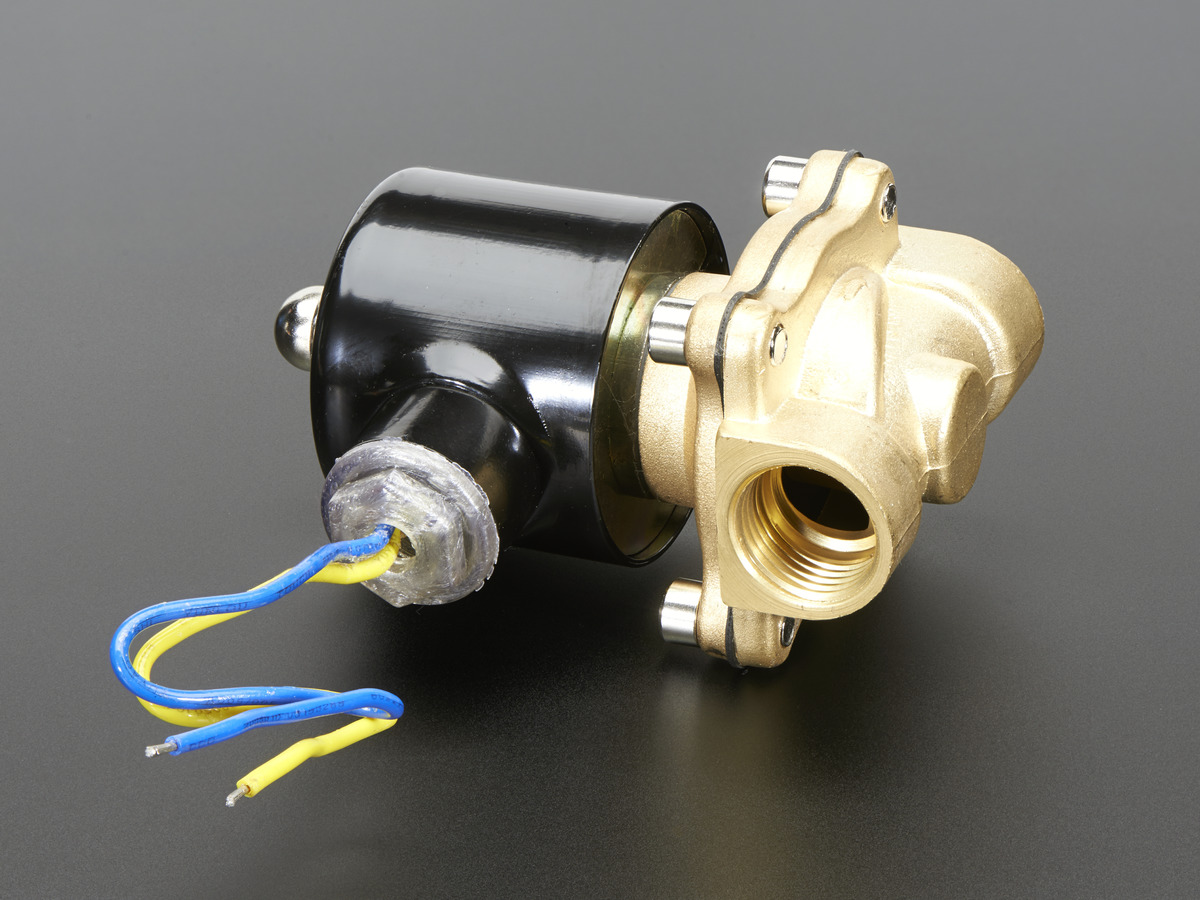
Figure 3: Valve image from specification sheet [2]
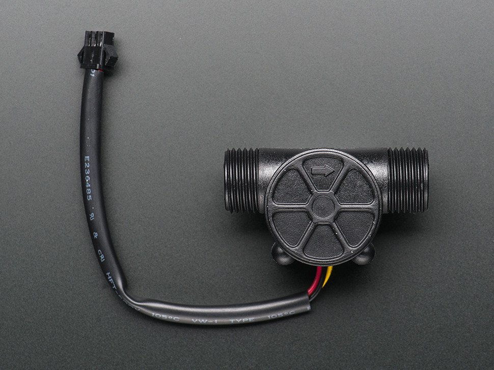
Figure 4: Flowmeter image from specification sheets [3]
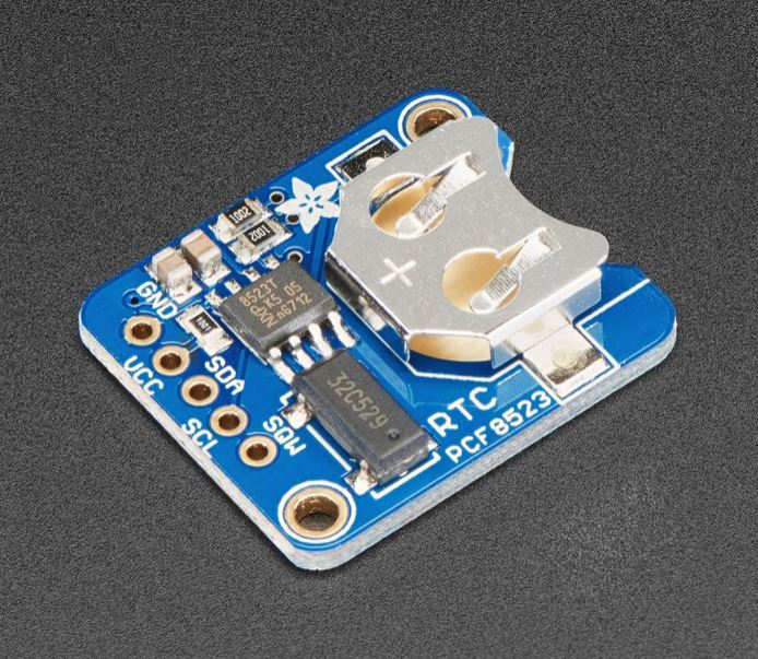
Figure 5: Real time clock image from specification sheets [4]
While we were designing the entire system, we were simultaneously testing individual components. During the previous week, we had problems with the relay. We initially thought that pi was not drawing enough current to register differences between digital high/low on the relay, so we tried operating the relay with an arduino and corresponding source code on a spec sheet we found online [5], which simply cycled through flipping each relay and lighting up the corresponding on-board LEDs. This worked, and after analyzing the arduino code provided, we realized that the relay clicked on when the arduino output digital low to the device. Accordingly, we tried using the relay with the raspberry pi, connecting its source voltage to 5V (again, as detailed on the spec sheet) and turning it on by driving its signal input digital low and it worked as expected. Earlier, we were working with a 4-relay array, and this week we switched it out with a single 5V relay Professor Skovira had on hand for compactness, and we found it worked the same way.
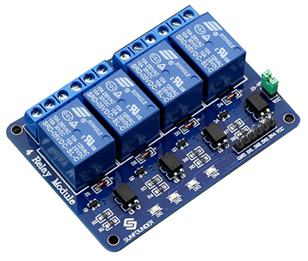
Figure 6: Image of relay array from specification sheet [5]
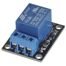
Figure 7: Image of single relay from specification sheet [6]
Week 3
This week, we received the flowmeter and the real time clock so we spent time learning how they worked and unit testing them. To test the flowmeter, we wrote a python script valve2.py that accepts input from the flowmeter via pin 20 with the line GPIO.setup(20, GPIO.IN, pull_up_down=GPIO.PUD_UP). Each time a falling edge of a pulse is detected, the callback function is called from the line GPIO.add_event_detect(20,GPIO.FALLING,callback=GPIO20_callback). The function GPIO20_callback() increments a global variable numiter that closes the valve via the relay (using the GPIO call GPIO.output(relay,GPIO.HIGH), where relay is the relay pin number) once a maximum number of iterations, maxiter, is reached. From the technical specifications of the flowmeter [4], there is a pulse each time 2.5 mL of liquid has passed through the flowmeter, thus, the amount of liquid flowing through the flowmeter = 2.5mL * number of interrupts. In place of water, we tested the flowmeter by blowing air directly into it.
Additionally, as mentioned before we wanted our irrigation process to start reliably at the same time every day, so we attempted to integrate the realtime clock in the process mentioned above. To get the clock working, we needed to set up i2c communication and install some libraries on the kernel including i2c detect, which displays all slaves on the SCL/SDA bus controlled by the RPi [7]. A screenshot of the output when the realtime clock was connected is displayed below - note that the real time clock’s default address is 68.
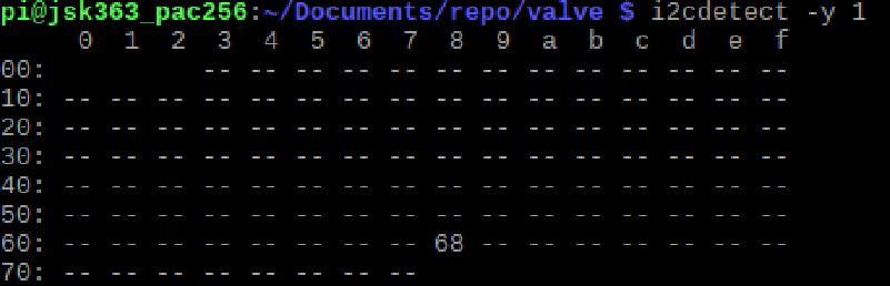
Figure 8: Screenshot of output from i2cdetect with the real time clock on the bus. There is a detected device on its default i2c address 68.
We also installed the python library smbus and were able to unit test the real time clock, reading from addresses on the i2c bus that contained running second/minute counters and interrupt flags. However, when using this library, we realized that there was no good way to have the real time clock interrupt the CPU (i.e. when starting our process at the same time everyday), since typically slaves cannot interrupt masters on an i2c bus, as the master sets the clock and can choose to ignore slaves’ transmissions on the bus. Instead, we took the route of setting up the real time clock as the source for our kernel’s internal timing module instead of the network time protocol (NTP, which requires an internet connection). Following directions we found on the internet [7], we allowed i2c interfacing in raspi-config, added the line dtoverlay=i2c-rtc,pcf8523 to our /boot/config.txt file (since we’re using the PCF8523 real time clock), and configured the hwclock so that it would no longer use the aptly-named fake-hwclock and instead use the i2c real time clock, which we were able to confirm was in fact working by disconnecting from the internet and issuing the date command.
Since the system needs to be exact with the amount of water it irrigates in addition to the fact that the bucket is wide and that amount of irrigated water during a given cycle could be small, we needed a way to ensure that all the water that flows into the bucket from the flowmeter exits the bucket. To accomplish this task, we thought about just tilting the bucket using bricks. This simple solution would solve the problem, but it is dependent on arranging bricks in the same orientation each time and carrying around bricks could be a burden. Instead, we 3D printed a part to put inside the bucket that directs all water to a hole in the bucket. Using CAD solidworks, we created a cylinder that sits in the bottom of the bucket. The part is slanted on the top as to direct all the water through a hole in the side of the bucket.
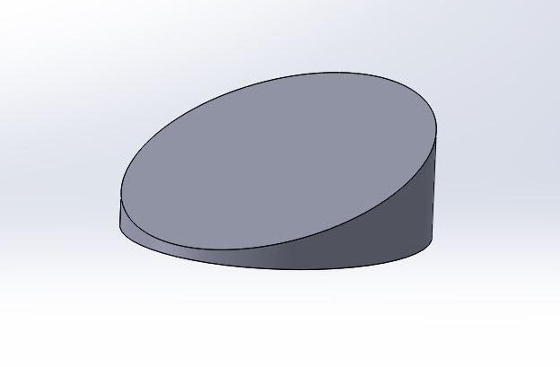
Figure 9: Our part shown in CAD solidworks
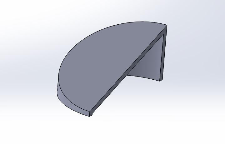
Figure 10: The profile of the part, showing how it is hollow on the inside.
One problem we had with the 3D printed part was that it was too big for the printer. We just cut the part in half on solidworks and printed the two halves separately. Then, we used epoxy to glue the parts together. Additionally, the 3D printed material used was not waterproof. This is a big problem because the part will be sitting under pooled water. To get around this, we painted the part with epoxy, which is waterproof. Finally, we placed the part in the bucket and sealed it using silicone caulk.
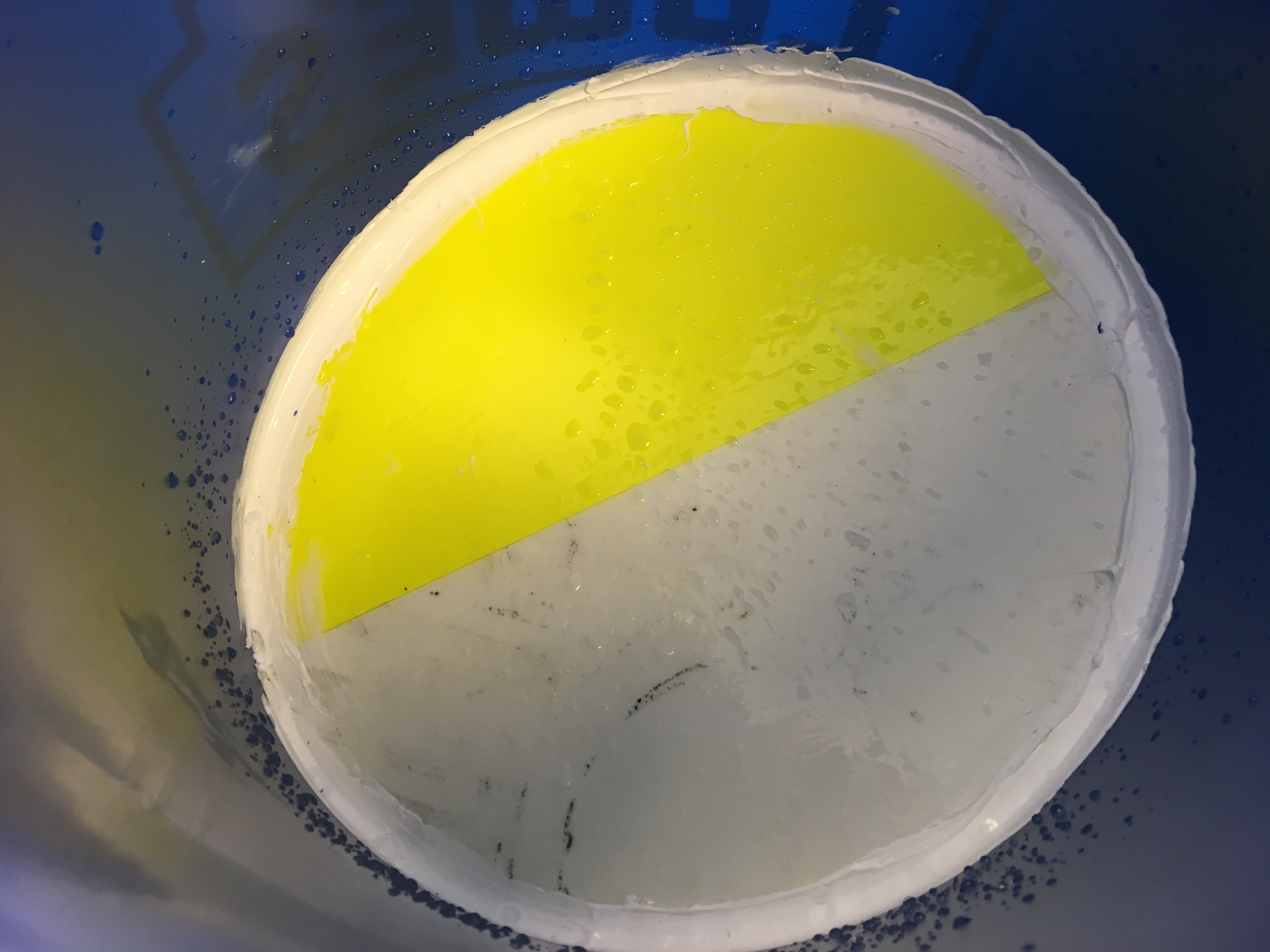
Figure 11: Our 3D printed part, glazed with epoxy and secured into place using silicon caulk
Next, we drilled a hole in the bucket for water to flow out of it and to the tree. We used a simple drill to cut a hole right above the 3D printed part so no water would get caught below the hole. After we used epoxy to attach a plastic water pipe nozzle. This allowed us to connect a hose to the bucket via the nozzle so water could flow from the bucket. Below are two videos. The first shows how easily water can flow out of the bucket through the nozzle. The second shows how the 3D printed parts allows the bucket to completely drain all water from it.
Figure 12: Video showing waterproof testing of the bucket
Figure 13: Video showing the bucket draining completely.
Week 4
This week, we began to assemble the final design, consolidate our code with the algorithm for determining the irrigation parameter [8], set it up to start at the same time every day, and perform integration tests. We were told that typically, water does not need to be irrigated during the nighttime since the water potential is relatively constant during this time period, but will change quite a bit during the daytime from about 6am to 10pm, so we needed to run the irrigation code for the entirety of this range each day. Our approach to solving this problem was to have the OS start our script using a crontab call every day at 6am, and to change some parameters in the code:
- dtODE: This parameter indicates the length of the timestep used for numerical integration in seconds. For testing, we set this value to 120 = 2 minutes.
- i: This parameter indicates the time of day which the algorithm should start (i.e. the start of the weather and pressure data it should fetch) as the number of timesteps dtODE since midnight. Since we wanted to start at 6am, we set this parameter to 6*3600/dt = 180.
- xexpected: This parameter functions as the initial value used for the numerical integration. For this application, we set this to [[-1,-1]] (real and imaginary parts).
- con: This parameter is the constraint on water pressure - the absolute value of the water pressure must be kept smaller than this value. For testing in the lab, we set this variable to -.97, very close to the initial value xexpected so that we would not have to irrigate large amounts of water in the lab and possibly make a mess.
- limit: This parameter indicates the time of day which the algorithm should terminate as the number of timesteps timesteps dtODE since midnight. For testing, we set this to i+10 so that our integration tests would be short, but in practice we would set this parameter to 22*3600/dt = 180, so the algorithm would terminate at 10pm.
Originally, the code already contained a call to a stub function irrigate(amount), which we implemented directly in the same file. As before, we set up the valve and flowmeter GPIO pins and interrupts in the same python script which we renamed irrigation_algorithm.py. Our irrigate function simply had to open the valve, driving the relay digital low, and change the max number of interrupts counted before closing the valve (a global variable maxiter to amount/.0025) based on the value of amount in liters and reset the current number of iterations (a global variable numiter) to 0. Then, we adapted the flowmeter ISR to drive the relay high when the max number of iterations was reached, and do nothing if numiter > maxiter. For testing, we printed the number of remaining iterations from the flowmeter interrupt ISR and saw that it was working properly when we blew into the flowmeter for different amounts. We accordingly were able to print the amount of water dtODE*u1/p (recall u1 was the rate of irrigation for the next iteration in kg/s and p was the density of water in kg/L) for each iteration of the numerical integration and print it to a log file, calling the script as python3.5 irrigation_algorithm.py > irrigationlog.txt so that we could keep a running record of the amount irrigated in each timestep in the file irrigationlog.txt. Note that the version of python being used is different from our RPi’s default, since the algorithm developed uses several libraries exclusive to python 3 which we needed to install on our system for this code to run properly.
To start the script at 6am every day, we used crontab, a time-based job scheduler that can run various commands starting processes at desired times of day or once every given interval. Since we had the system clock synchronized with the i2c real time clock module, we could be sure that this scheduling would be precise. To execute our python script from crontab, we initially had to make the script executable from anywhere. We achieved this by adding pound-bang interpreter directive #!/usr/bin/env python3.5 to the very start of the script and allowing all users permission to execute with the command chmod +x irrigation_algorithm.py. The result of these changes was that the script could be directly executed from the command line using python 3 with the simple syntax ./irrigation_algorithm.py. Then, we added a line to our crontab file, /etc/crontab.
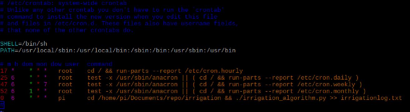
Figure 14: Screenshot showing the line we added to our crontab file, which calls irrigation_algorithm.py and appends the output to irrigationlog.txt at 6am every day as user pi.
The last line indicates that at the 0th minute of the 6th hour of every day and month, the user pi will change directory to the folder that contains our script (necessary for the script to load all required files) and execute it, concatenating all outputs (amounts irrigated) to the text file irrigationlog.txt. Initially, we had some problems getting this to work since the code output to the text file perfectly well from the command line but appeared to be wiping it clean when it was started with crontab. To test this, we added a crontab call to a temporary second script every minute (i.e. by making the first few columns to 0-59 * * *) and began adding our code to this script in small pieces so we could see exactly what was making it not work in crontab. We found that a try...except block we had wrapped the main loop in to halt execution on a KeyboardInterrupt was the reason it was not working, perhaps because flowmeter interrupts were ceasing execution in a different setting. Either way, we removed this construct and it began working exactly as expected.
In the process of assembling the final design, we placed the valve and flowmeter into a plastic container. The purpose of this was to keep the outside of the components and the wires coming from the components dry in case the water source ever leaked. We cut holes in the containers for the water to go in and out of the components and then sealed the holes using silicone caulk.
Then we performed waterproofing tests. Essentially, we opened the valve and poured water through the valve and flowmeter to see if water got into the container. Water did no so the box was waterproof.
Next, we were ready to test with a hose; however, we did not have a hose or a water source near the required power supplies to power the valve and flowmeter. To get around this, we filled another container with water and placed it above the valve.
The largest problem we had was the flowmeter did not work as we expected. In our initial design, we had the water supply connected to the valve and then to the flowmeter. In an integration test, we used valve2.py to test the system. Once the valve was open, we measured out exactly 250mL and started to pour the water into the valve. The valve consistently closed after only a small fraction of the 250mL was poured through the system. We next changed the maximum number of iterations so different amounts of water would be irrigated. Still, a far too small amount of water was consistently irrigated.
We then detached the flowmeter and connected the output of the flowmeter to an oscilloscope. Then, we blew in the flowmeter to see what the pulses look like. Below is a video of the oscilloscope sensing the output. As expected after a large breath of air is blown, the flowmeter sent many pulses quickly and then the rotor slows down and there are more time between pulses on the oscilloscope . Below is the video.
Figure 15: Flowmeter interrupt signal displayed on the oscilloscope, blowing into the opening.
We found out that each time we opened the valve, water initially mixed with the air in the flowmeter flowed through the flowmeter. Because of this, the flowmeter was reading that a lot more water was flowing through the flowmeter than what was actually flowing through the flowmeter.
We then decided that we concluded that the flowmeter should always be full of water so no air would be going through the flowmeter, making our measurements incorrect. To do this, we flipped the valve and flowmeter so the water travelled from the source through the flowmeter and then through the valve.
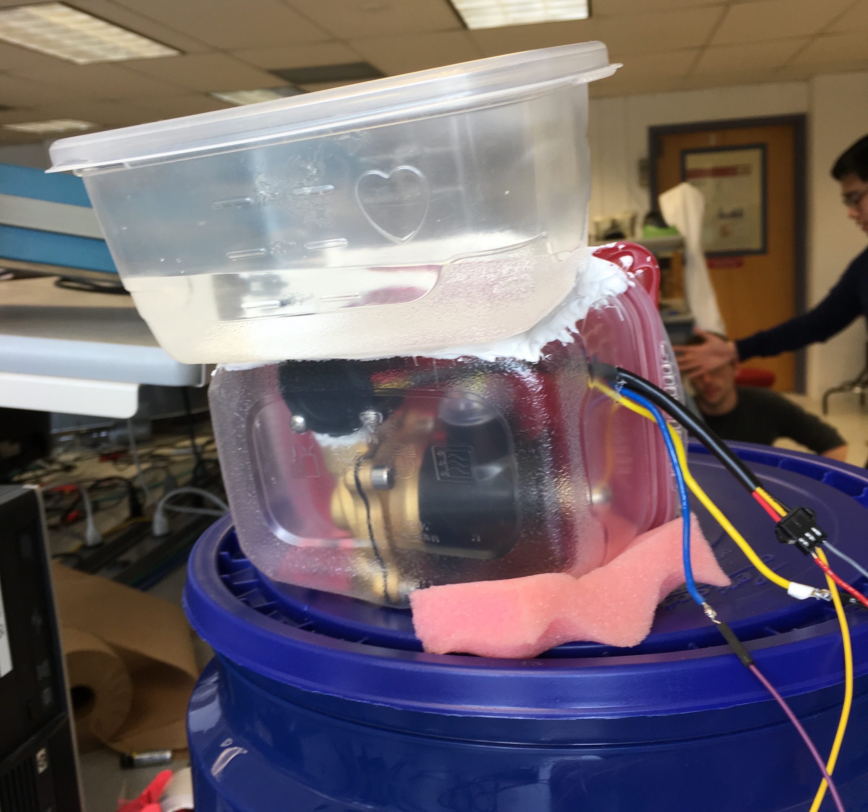
Figure 16: Out reservoir setup on top of the flowmeter so that the flowmeter would remain full of water at all times.
We then tested this new idea. Unfortunately, this did not solve the problem. We set up the system to irrigate a liter of water and just tens of milliliters came out. We then thought that maybe the flowmeter needed to be calibrated and that the measurements would be consistently off by a linear amount. This was also not the case. After testing many different amounts of water, we determined that the flowmeter was extremely inconsistent.
At this same time, the flowmeter broke. It completely stopped sending any output pulses. We thought we had plugged it into the wrong pin or something, but after investing, our circuitry was correct. We then connected the output of the flowmeter to the oscilloscope and blew into the flowmeter. There were no pulses.
Since this happened the day of our demo, we decided to scrap the flowmeter altogether and see if there was a linear relationship between the amount of water that could flow through the valve and on the amount of time the valve was open for. After varying the amount of time the valve was open for (between 0.5 and 3 seconds) and measuring the water output, we found there was a linear relationship.
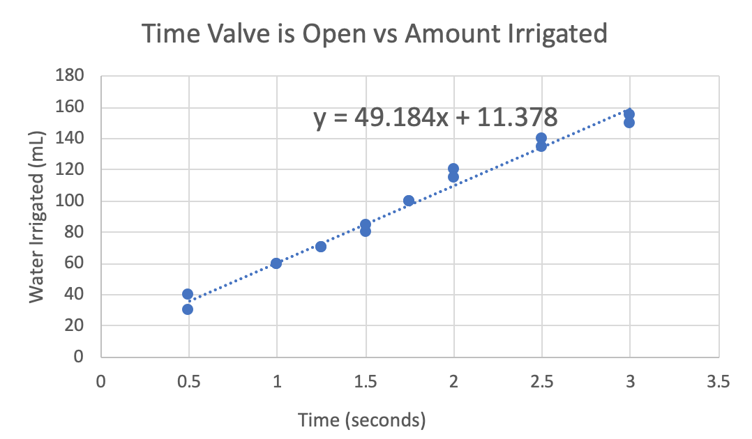
Figure 17: Graph of the measured amount of water irrigated versus the amount of time we kept the valve open for. Inscribed is the equation of best fit.
Experimentally, we found that opening the valve for 1.75 seconds extremely consistently irrigated 100 mL of water. As a result, we made a new file, irrigation_algorithm.py, which uses just the valve to irrigate water and renamed the file that uses the flowmeter to irrigate to irrigation_algorithm_prev.py. In this file, we decided that each irrigation cycle, we would irrigate 100 mL, and the carryover would be irrigated in future irrigation cycles. Because the amount of water to irrigate decreases to zero after just a couple irrigation cycles, all water was always able to be irrigated within about 4 cycles. When the amount of water is less than 100 mL, we calculated the time to open the valve for from the best fit line of the data points. Since the amount of water irrigated = [(49.184* time the valve is open for) + 11.378] mL, we found that we should open the valve for [(amount of water in mL - 11.378)/49.184] seconds. This method allowed us to accurately irrigate small amounts of water (small amounts because we only have the plastic containers worth of water with the current set up). Below is our final demo which shows the working system.
Figure 18: Final project demo in the lab
Results
Over the course of these last few weeks, we ran into difficulties with almost all of the parts we bought or were given. First, we had issues with the relay, we didn’t know how to use the real time clock initially, and the flowmeter ended up breaking on the day of our presentation. Though we were able to overcome most of these obstacles and still produce something that was a good lead on our final goal, there were some shortcomings in what we demoed in the lab. Our system, though it does reliably irrigate small amounts of water, it will have trouble running autonomously when it needs to irrigate larger amounts of water or operate for a longer period of time. This is partially due to the fact that we did not know where to get a hose, so we opted to use a small reservoir that in practice would have to be manually refilled once empty. We also did not get into the software part of this project we initially described, which would fetch weather forecast data from the internet and water potential data from an IoT-based data logger necessary as inputs parameters for the irrigation algorithm, since we ran out of time. However, our completed system does reliably begin to irrigate small amounts of water at 6am ending at 10pm every day, and output those amounts to a log file for future use. In that sense, we completed most of the physical design (if we tinkered with a hose and flowmeter that worked reliably, we would have completed all of it) and the software part of this project could easily be added on later.
Conclusion
We created an irrigation system that is able to accurately measure and irrigate water amounts determined by the algorithm given to us by our friends in the chemical engineering department. We successfully integrated software and multiple electrical components, such as the relay, flowmeter, real time clock, and solenoid valve, with the raspberry pi to get our project to work. In the process, we realized how bold it was to bring water into and electrical engineering lab. Waterproofing is difficult and mistakes can easily destroy equipment; however, we were able to use simple equipment to fully waterproof our system. We also discovered that it is worth investing in high quality parts. Our flowmeter failed which could have been detrimental to our project. Additionally, it did not work as expected even when it was functional. We also were quite ambitious with the amount of work that we took on. We did not have time to collect data from the IoT and from weather forecasting sources for the main algorithm as we did not realize how complicated it would be to integrate all the components together when making the main system and how many unexpected errors arose while we worked. All in all, we were successful with our main objective from the beginning and we have provided a strong platform for the project to continue to grow for Corentin and Rui.
Future Work
In the future, we would first try buying a different flowmeter and hopefully see some discernible improvement in its operation over the one we bought. We would also buy other plumbing connectors so that we could test this new flowmeter when directly connected to a hose, making sure that the pressure in the hose does not change the accuracy of its pulses too much, or otherwise calibrate to a constant pressure in the hose. We kept our old code that registers flowmeter interrupts, so this step would only take a few hours of testing in theory. Additionally, since the project will be in the field exposed to the elements, there likely needs to be structurally sound housing for the raspberry pi and the circuit components to protect it all. This would involve buying or 3D printing other parts, and caulking it all together as we did in what we demoed. In the same vein, we could also use batteries instead of the dc power supply we use in the lab. Finally, we could take care of the software element that reads weather data from the internet and water potentials from the IoT platform - the former would be relatively easy as long as we can secure an internet connection for a short period of time before 6am every day (possibly through a cellular overlay, which might involve buying a radio transceiver), and the latter would likely require some work interfacing with the IoT. The result of these further improvements would be a fully autonomous system that regulates tree water potential completely disconnected from external power sources, internet connections, and does so reliably without any worry of weather conditions destroying our setup; the only intervention required would be switching batteries every once in a while.
Code Appendix
1 2 3 4 5 6 7 8 9 10 11 12 13 14 15 16 17 18 19 20 21 22 23 24 25 26 27 | # Final Project: valve.py # May 13, 2019 # Authors: Jackson Kopitz jsk363, Peter Cook pac256 import RPi.GPIO as GPIO import time import numpy as np import subprocess valve = 16 GPIO.setmode(GPIO.BCM) #broadcom numbering GPIO.setup(valve, GPIO.OUT) GPIO.output(valve, GPIO.LOW) high = False try: while True: time.sleep(5) if high: GPIO.output(valve, GPIO.LOW) high = False else: GPIO.output(valve, GPIO.HIGH) high = True except KeyboardInterrupt: GPIO.cleanup() |
1 2 3 4 5 6 7 8 9 10 11 12 13 14 15 16 17 18 19 20 21 22 23 24 25 26 27 28 29 30 31 32 33 34 35 36 37 38 39 40 41 42 43 44 45 46 | # Final Project: valve2.py # May 13, 2019 # Authors: Jackson Kopitz jsk363, Peter Cook pac256 import RPi.GPIO as GPIO import time import numpy as np import subprocess relay = 16 GPIO.setmode(GPIO.BCM) #broadcom numbering GPIO.setup(relay, GPIO.OUT) numiter = 0 maxiter = 100 def GPIO20_callback(channel): """on flowmeter interrupt, increase vol by 2.5mL. if desiredvol reached, close valve""" global numiter global maxiter if numiter == 0 and maxiter > 0: numiter += 1 print(numiter) elif numiter < maxiter and maxiter > 0: numiter += 1 print(numiter) elif numiter == maxiter: GPIO.output(relay, GPIO.HIGH) numiter += 1 else: print("Valve should be closed now!") GPIO.setup(20, GPIO.IN, pull_up_down=GPIO.PUD_UP) GPIO.add_event_detect(20,GPIO.FALLING,callback=GPIO20_callback) GPIO.output(relay, GPIO.LOW) try: while True: time.sleep(1) except KeyboardInterrupt: GPIO.cleanup() exit() |
1 2 3 4 5 6 7 8 9 10 11 12 13 14 15 16 17 18 19 20 21 22 23 24 25 26 27 28 29 30 31 32 33 34 | # Final Project: testrtclock.py # May 13, 2019 # Authors: Jackson Kopitz jsk363, Peter Cook pac256 # test script when attempting to get the real time clock # to work with interrupts using python libraries import RPi.GPIO as GPIO import time import numpy as np import subprocess import smbus channel = 1 #using i2c channel 1 for the realtime clock - labeled scl,sda addr = 0x68 #default i2c address of i2c clock bus = smbus.SMBus(channel) # Initialize I2C (SMBus) #control status register 0x00 controlstatus0 = bus.read_byte_data(addr,0x00) #bus.write_byte(addr, controlstatus0 | 0b00000100) #enable second interrupts #don't know if interrupts are going to work initseconds = bus.read_byte_data(addr,0x03) #"seconds" register now = 0 print(initseconds) #try polling try: while True: now = bus.read_byte_data(addr, 0x04) print(now) except KeyboardInterrupt: GPIO.cleanup() exit() |
1 2 3 4 5 6 7 8 9 10 11 12 13 14 15 16 17 18 19 20 | # Final Project: testcrontab.py # May 13, 2019 # Authors: Jackson Kopitz jsk363, Peter Cook pac256 # file to test the cron tab #!/usr/bin/python import subprocess import RPi.GPIO as GPIO import time relay = 16 GPIO.setmode(GPIO.BCM) #broadcom numbering GPIO.setup(relay, GPIO.OUT) GPIO.setwarnings(False) GPIO.output(relay, GPIO.HIGH) time.sleep(5) GPIO.output(relay, GPIO.LOW) GPIO.cleanup() |
1 2 3 4 5 6 7 8 9 10 11 12 13 14 15 16 17 18 19 20 21 22 23 24 25 26 27 28 29 30 31 32 33 34 35 36 37 38 39 40 41 42 43 44 45 46 47 48 49 50 51 52 53 54 55 56 57 58 59 60 61 62 63 64 65 66 67 68 69 70 71 72 73 74 75 76 77 78 79 80 81 82 83 84 85 86 87 88 89 90 91 92 93 94 95 96 97 98 99 100 101 102 103 104 105 106 107 108 109 110 111 112 113 114 115 116 117 118 119 120 121 122 123 124 125 126 127 128 129 130 131 132 133 134 135 136 137 138 139 140 141 142 143 144 145 | # Final Project: irrigation_algorithm_prev.py # May 13, 2019 # Authors: Jackson Kopitz jsk363, Peter Cook pac256 #!/usr/bin/env python3.5 from scipy import integrate as integ import numpy as np from solvers import linearODEgetUAppleStWP, OdeFunctionApple2 import matplotlib.pyplot as plt from Fetch_weather_data import get_Precip from hardware_control import irrigate from SpeedUp import get_ET_speed, get_ET_speed_max from Data_apple_tree import * import time import RPi.GPIO as GPIO import subprocess #our initializations numiter = 1 maxiter = 0 relay = 16 flowmeter = 20 GPIO.setmode(GPIO.BCM) #broadcom numbering GPIO.setup(relay, GPIO.OUT) GPIO.setup(flowmeter, GPIO.IN, pull_up_down=GPIO.PUD_UP) def GPIO20_callback(channel): """on flowmeter interrupt, increase vol by 2.25mL. if desiredvol reached, close valve""" global numiter global maxiter if numiter == 0 and maxiter > 0: numiter += 1 #print(numiter) elif numiter < maxiter and maxiter > 0: numiter += 1 #print(numiter) elif numiter == maxiter: GPIO.output(relay, GPIO.LOW) numiter += 1 else: print("Valve should be closed now!") GPIO.add_event_detect(flowmeter,GPIO.FALLING,callback=GPIO20_callback) def irrigate(amount): """irrigates the amount of water by setting global variables to be handled by the ISR and opening the valve""" global numiter global maxiter global relay numiter = 0 maxiter = int(amount / 0.0025) printstr = "Maxiter is " + str(maxiter) print(printstr) GPIO.output(relay, GPIO.HIGH) #### MPC initializations horizon=1000 H_ODE = 10 # prediction horizon con = -.97 # constraint for trunk water potential (bar) irMax = 1 # irrigation rate maximum (kg/s) pen = 1 # penalty weight for slack variable dtODE=120 # every two minute dtForecast= 3600 # forecast every hour time_horizon_Ode=dtODE*np.array(range(H_ODE+int(dtForecast/dtODE))) H_Forecast=2+int(H_ODE*dtODE/dtForecast) time_horizon_Forecast=dtForecast*np.array(range(H_Forecast)) x0_real=[] ureal = [] xreal = [] xexpected=[[-1,-1]] experiment_running=True i=180 #(i will be suppressed in real experiments) limit=190 ET_real=[] t=time.time() numdts = 5 #irrigate every 10 minutes curdts = 1 curamt = 0 totamt = 0 while experiment_running: ETforecast=get_ET_speed(H_Forecast,i//int((dtForecast/dtODE)), xexpected[-1][0]) #(i will be suppressed in real experiments) # ETforecast for the H next hours ETforecast2=get_ET_speed_max(H_Forecast,i//int((dtForecast/dtODE))) #(i will be suppressed in real experiments) #ETforecast for the H next hours Precipforecast=get_Precip(H_Forecast,i//int((dtForecast/dtODE))) #(i will be suppressed in real experiments) #Precipe forecast for the H next hours ETODE=np.interp(time_horizon_Ode[i%int((dtForecast/dtODE)): i%int((dtForecast/dtODE))+H_ODE],time_horizon_Forecast,ETforecast) ETODE2=np.interp(time_horizon_Ode[i%int((dtForecast/dtODE)): i%int((dtForecast/dtODE))+H_ODE],time_horizon_Forecast,ETforecast2) ET_real.append(ETODE[0]) PrecipODE=np.interp(time_horizon_Ode[i%int((dtForecast/dtODE)): i%int((dtForecast/dtODE))+H_ODE], time_horizon_Forecast,Precipforecast) xreal.append(x0_real) # x0_real=get_x0(x0_real) #Normal way of writing x0_real=xexpected[-1] u1 = linearODEgetUAppleStWP(np.matrix(x0_real), ETODE2,PrecipODE, Rr,Rt,Ct,Cs,r1,r2,RLD,Vs,rhow,as1,n,m,Ks,dtODE \ ,H_ODE, con, irMax, pen) ureal.append(u1) #u1 is irrigation rate in kg/s # dtODE is the amount of time to irrigate in seconds curamt += u1*dtODE if curdts < numdts: curdts += 1 curamt += u1*dtODE else: irrigate(curamt) curdts = 1 curamt = 0 time.sleep(dtODE/12) #In case we're not measuring the water potential water = u1 + PrecipODE[0] y = integ.odeint(OdeFunctionApple2, np.array(x0_real), [0,dtODE], (ETODE[0], water, \ Rr,Rt,Ct,Cs,r1,r2,RLD,Vs,rhow,as1,n,m,Ks)) xexpected.append(y[1]) # print("xodeint=",xexpected[-1]) i+=1 if i>=limit-1: experiment_running=False print("Total amount irrigated = " + str(totamt)) t = time.time() - t print("Execution = " + str(t)) GPIO.cleanup() |
1 2 3 4 5 6 7 8 9 10 11 12 13 14 15 16 17 18 19 20 21 22 23 24 25 26 27 28 29 30 31 32 33 34 35 36 37 38 39 40 41 42 43 44 45 46 47 48 49 50 51 52 53 54 55 56 57 58 59 60 61 62 63 64 65 66 67 68 69 70 71 72 73 74 75 76 77 78 79 80 81 82 83 84 85 86 87 88 89 90 91 92 93 94 95 96 97 98 99 100 101 102 103 104 105 106 107 108 109 110 111 112 113 114 115 116 117 118 119 120 121 122 123 124 125 126 | # Final Project: irrigation_algorithm.py # May 13, 2019 # Authors: Jackson Kopitz jsk363, Peter Cook pac256 #!/usr/bin/env python3.5 from scipy import integrate as integ import numpy as np from solvers import linearODEgetUAppleStWP, OdeFunctionApple2 import matplotlib.pyplot as plt from Fetch_weather_data import get_Precip from hardware_control import irrigate from SpeedUp import get_ET_speed, get_ET_speed_max from Data_apple_tree import * import time import RPi.GPIO as GPIO import subprocess #our initializations numiter = 1 maxiter = 0 relay = 16 flowmeter = 20 GPIO.setmode(GPIO.BCM) #broadcom numbering GPIO.setup(relay, GPIO.OUT) def irrigate(amount): """irrigates the amount of water by setting global variables to be handled by the ISR and opening the valve""" global numiter global maxiter global relay thistime = (amount/.001 - 11.378)/49.184 GPIO.output(relay,GPIO.HIGH) time.sleep(thistime) #1mL/.1s GPIO.output(relay,GPIO.LOW) #### MPC initializations horizon=1000 H_ODE = 10 # prediction horizon con = -.97 # constraint for trunk water potential (bar) irMax = 1 # irrigation rate maximum (kg/s) pen = 1 # penalty weight for slack variable dtODE=120 # every two minute dtForecast= 3600 # forecast every hour time_horizon_Ode=dtODE*np.array(range(H_ODE+int(dtForecast/dtODE))) H_Forecast=2+int(H_ODE*dtODE/dtForecast) time_horizon_Forecast=dtForecast*np.array(range(H_Forecast)) x0_real=[] ureal = [] xreal = [] xexpected=[[-1,-1]] experiment_running=True i=180 #(i will be suppressed in real experiments) limit=190 ET_real=[] t=time.time() numdts = 5 #irrigate every 10 minutes curdts = 1 curamt = 0 totamt = 0 max_to_irrigate=.1 while experiment_running: ETforecast=get_ET_speed(H_Forecast,i//int((dtForecast/dtODE)), xexpected[-1][0]) #(i will be suppressed in real experiments) #ETforecast for the H next hours ETforecast2=get_ET_speed_max(H_Forecast,i//int((dtForecast/dtODE))) #(i will be suppressed in real experiments) #ETforecast for the H next hours Precipforecast=get_Precip(H_Forecast,i//int((dtForecast/dtODE))) #(i will be suppressed in real experiments) #Precipe forecast for the H next hours ETODE=np.interp(time_horizon_Ode[i%int((dtForecast/dtODE)): i%int((dtForecast/dtODE))+H_ODE],time_horizon_Forecast,ETforecast) ETODE2=np.interp(time_horizon_Ode[i%int((dtForecast/dtODE)): i%int((dtForecast/dtODE))+H_ODE],time_horizon_Forecast,ETforecast2) ET_real.append(ETODE[0]) PrecipODE=np.interp(time_horizon_Ode[i%int((dtForecast/dtODE)): i%int((dtForecast/dtODE))+H_ODE], time_horizon_Forecast,Precipforecast) xreal.append(x0_real) # x0_real=get_x0(x0_real) #Normal way of writing x0_real=xexpected[-1] u1 = linearODEgetUAppleStWP(np.matrix(x0_real), ETODE2, PrecipODE, Rr,Rt,Ct,Cs,r1,r2,RLD,Vs,rhow,as1,n,m,Ks,dtODE \ ,H_ODE, con, irMax, pen) ureal.append(u1) #u1 is irrigation rate in kg/s #dtODE is the amount of time to irrigate in seconds totamt += u1*dtODE curamt += u1*dtODE print(curamt) if curamt > max_to_irrigate: irrigate(max_to_irrigate) curamt -= max_to_irrigate elif curamt > 0: irrigate(curamt) curamt = 0 time.sleep(dtODE/12) #In case we're not measuring the water potential water = u1 + PrecipODE[0] y = integ.odeint(OdeFunctionApple2, np.array(x0_real), [0,dtODE],(ETODE[0], water, \ Rr,Rt,Ct,Cs,r1,r2,RLD,Vs,rhow,as1,n,m,Ks)) xexpected.append(y[1]) # print("xodeint=",xexpected[-1]) i+=1 if i>=limit-1: experiment_running=False print("Total amount irrigated = " + str(totamt)) t = time.time() - t print("Execution = " + str(t)) GPIO.cleanup() |
Budget
Total = $71.76
- Raspberry Pi - free
- Bucket - $3.25
- Bucket Lid - $1.68
- 3D Printed Part - $5
- Plastic Tubing - $8.98
- Silicone Caulk - $5
- Epoxy - $3
- Plastic Pipe Nozzle - $2
- Solenoid Valve - $24.95
- Flowmeter - $9.95
- Real Time Clock Module - $4.95
- Resistors and Wires - $1.00
- Plastic Containers - $2.00
- Water - free
Work Distribution
Jackson
Objective, half of each Week 1-4, Conclusion, Budget, and Website
Peter
Introduction, half of each Week 1-4, Result, Future Work, and References
References
[1] Efficient Irrigation Control for Tree Trunk Water Potential Through Model Predictive Control, Wei-Han Chen and Fenhqi You, www.peese.org
[2] Brass Liquid Solenoid Valve - 12V - ½ NPS, Adafruit, https://www.adafruit.com/product/996
[3] Liquid Flow Meter - Plastic ½” NPS Threaded, Adafruit, https://www.adafruit.com/product/828
[4] Adafruit PCF8523 Real Time Clock Assembled Breakout Board, Adafruit, https://www.adafruit.com/product/3295
[5] 4 Channel 5V Relay Module, Sunfounder Wiki, http://wiki.sunfounder.cc/index.php?title=4_Channel_5V_Relay_Module
[6] Arduino Compatible 5V Relay Board, Jaycar, https://www.jaycar.us/arduino-compatible-5v-relay-board/p/XC4419
[7] Raspberry Pi RTC: Adding a Real Time Clock, PiMyLifeUp, Gus, https://pimylifeup.com/raspberry-pi-rtc/
[8] Irrigation Algorithm apple_npc.py, Corentin Bisot
Contact
Jackson Kopitz, jsk363@cornell.edu
Peter Cook, pac256@cornell.edu