Digital Guitar Effects Box
Christian Ray (cdr85) and Ben Roberge (bjr73)
May 15, 2019
Our Final System
Introduction
Instrument effects are ubiquitous in this modern era of music, from the signature "wah-wah" solos of Jimi Hendrix to the legendary classic rock distortion of Jimmy Page. These effects give life and character to the otherwise unassumingly calm and clean electric guitar. By modifying the analog audio output of an instrument in a certain way, musicians can craft signature sounds as well as entirely new genres.
Individual guitar effect pedals can range from $60 to $300 in price depending on the quality, type of effect, and number of adjustable parameters of the effect itself. The average electric guitarist can expect to use around four to eight of these pedals during live shows. After learning about the utility and low cost of modern embedded operating systems, we were inspired to use a Raspberry Pi to create a digital guitar pedal that could replicate several of these expensive guitar pedals.
We prioritized the end use of the guitar pedal when choosing which goals we wanted to meet with the pedal's design. First, we wanted the pedal itself to be standardized alongside other guitar pedals and compatible with the inputs and outputs commonly used by guitarists. This meant converting a 1/4" jack analog output signal from the electric guitar into a digital signal before manipulating it with the Raspberry Pi. After the audio effect modifications have been applied, the audio would then need to be converted back to an analog signal with a 1/4" output jack in order to enable it to be sent to a traditional guitar amplifier.
Secondly, we wanted to capitalize on some of the unique advantages and capabilities of the Raspberry Pi. We decided to incorporate a 320x240 pixel touchscreen from Adafruit to make a graphical user interface that would allow the user to intuitively navigate between effects.
Finally, we wanted our pedal to emulate real guitar pedals used in music production today. The effects
that we ultimately implemented are effects that are used worldwide in a variety of genres. Our effects
also incorporate adjustable parameters commonly used by other guitar pedals, such as the "delay time"
parameter used in delay effect pedals.
Objectives
The purpose of this project is to make a guitar effect pedal that allows a user to record a clip of audio, choose from a list of effects, and then set parameters for that effect before modifying the sampled audio clip itself. After the audio effect has been applied, the user will then be able to play back both the original and modified versions of the audio clip. Once the audio sample has finished playing, it will then be looped to repeat over and over again in the same vain as a looping backing track, or a backup rhythm guitarist. When the user is finished, he/she will be able to apply new effects to the clip or record a new audio sample.
Design
High Level Design
Our original project goal was to develop a fully functional guitar pedal, based on a
Raspberry Pi Model 3, with
a suite of custom effects. We wanted the system to process audio input in real-time and produce audio output
with as little latency as possible. We hoped to enable the system to apply several effects to the input signal,
with the understanding that time constraints would limit the number of effects we would be able to implement. We
understood that we would need some adapter to convert the 1/4" guitar jack output to a USB input that the
Raspberry Pi would be able to handle. We also needed an ADC before the input to the Raspberry Pi. On the output
side, we needed a DAC, as well as some way to convert the 3.5 mm output from the Raspberry Pi back to a 1/4"
cable that could connect to a standard guitar amplifier.
Another central goal was to create an intuitive user interface that would convey system information
to the user and enable the user to configure system parameters. We intended to use rotary encoders and push
buttons to enable user input and use a PiTFT screen to display system information for the user. Like many
guitar pedals, we planned to use one centrally-located push button to enable the effects.
When designing the system, we envisioned making a single, enclosed unit, like most standard guitar pedals.
We planned to make a simple, 3D-printed enclosure to house all the system hardware, with the exception of any
needed cables. Figure 1 shows the diagram we made of our system hardware when we submitted our project
proposal.
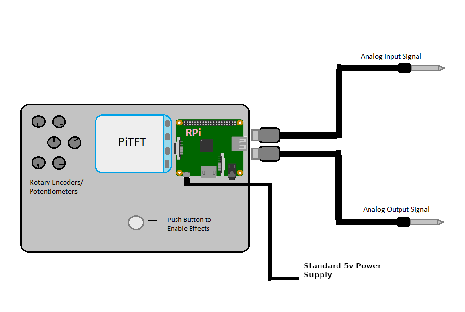
Figure 1: Diagram of Initially Proposed System
Effects Research
In order to decide which particular effects to implement, we needed to do some background research into the more common electric guitar effects. The following is a list of some of the effects we found, along with descriptions and examples.
Chorus
The Chorus effect emulates the effect naturally produced by choirs or orchestras where multiple tones of slightly different frequencies are mixed. A good example of Chorus is the intro to "Come as You Are" by Nirvana.
Phaser
A Phaser effect creates a rippling quality in the sound by dividing the audio signal into two and altering the phase of one portion. This effect can be clearly heard at the beginning of "Just the Way You Are" by Billy Joel.
Flanger
The Flanger effect has been described as a "jet plane" or "spaceship" sound. Traditionally, it was implemented by recording a track on two synchronized tapes and periodically slowing the playback of one tape by pressing on the edge of its reel (the "flange"). A Flanger effect can be heard right before the bridge in "Listen to the Music" by The Doobie Brothers.
Tremolo
The Tremolo effect is a rapid, subtle variation in the volume of a passage. A good example of Tremolo is the beginning of "Born on the Bayou" by Creedence Clearwater Revival.
Vibrato
The Vibrato effect is similar to Tremolo, except that Vibrato rapidly varies the pitch of a note or passage, instead of the volume. Vibrato mimics the fractional semitone variations produced by string instrument players and singers when sustaining a note. Vibrato can clearly be heard in the guitar solo in "Samba Pa Ti" by Carlos Santana.
Wah-wah
A Wah-wah pedal sweeps the passband of a filter up and down in frequency to create its signature "wah" sound. The opening of "Voodoo Child (Slight Return)" by Jimi Hendrix is famous for its use of "wah-wah."
Delay
The Delay effect produces an echoing sound by overlaying a time-delayed duplicate onto the original signal. It is sometimes referred to as the Echo effect. Delay is employed at the beginning of "Welcome to the Jungle" by Guns N' Roses.
Reverb
The Reverb effect duplicates the sounds produced in echo chambers by creating a large number of echoes that gradually decay or fade away. Reverb is applied to the drums in "When the Levee Breaks" by Led Zeppelin.
Distortion
Distortion, or Overdrive, effects are often thought of as "gain" effects. Traditionally, they were implemented by boosting the gain of the signal so much that the voltage rails of the amplifier "clipped" the signal. This "clipping" distorts the shape of the waveform and produces overtones. Distortion produces a sound that can be described as "gritty" or "fuzzy." It is used throughout "Revolution" by The Beatles.
Hardware Design
In order for the effect pedal to meet the input/output cable conventions of other effect pedals, it was necessary to design the hardware to be compatible with the standard 1/4" cable used in conveying audio output from guitar pickups. Additionally, the output audio signal from the effect pedal needed to be compatible with the 1/4" female jacks that are used in standard guitar amplifiers. Finally, the transmission of the signal itself needed to be converted from the analog signal coming from the guitar to a digital audio signal before being read and modified by the Raspberry Pi. All audio signals coming from guitars are mono signals, so we kept the entirety of the project in a mono audio format.
To satisfy both of the aforementioned input conditions, we purchased a
Behringer 1/4" jack to USB
interface cable with a built-in analog to digital converter (ADC). This provided the proper 1/4" jack to connect to
a standard guitar as well as a clean and easy way to transmit the signal to the Raspberry Pi with a USB port. It also
automatically converted the analog audio input into a digital signal. The built-in ADC could sample at up to 48 kHz and
had a bit depth of 16 bits.
For the transmitting audio from the Raspberry Pi to a guitar amplifier, we elected to use the Pi's built-in digital to
analog converter (DAC). Once the output signal had been passed through the DAC, it was output through the Pi's 3.5 mm
headphone jack. Then to transmit the audio signal from this 3.5mm female jack to the 1/4" female jack commonly used in
guitar amplifiers, we purchased a
VCE 3.5mm Male to 1/4" Female Jack Adapter.
We then connected this adapter to a guitar amplifier with a standard 1/4" male to male cable.
Almost all guitar pedals include some method to manipulate various parameters of audio effects to produce slightly
different custom sounds. For our pedal effect interface, we chose to build three
rotary encoders
into the housing of the pedal. We capped these rotary encoders off with a set of
knurled metal knobs.
Each of these rotary encoders uses two signal outputs to determine which direction the encoder is rotating. We
connected both signal outputs of each encoder to an unused GPIO pin on the Raspberry Pi. Finally, we connected the
three encoders to the common ground of the system. Another element used in our effect selection interface is the
2.8" PiTFT Touchscreen Display from Adafruit,
which we connected to the Raspberry Pi with a 40 pin ribbon cable.
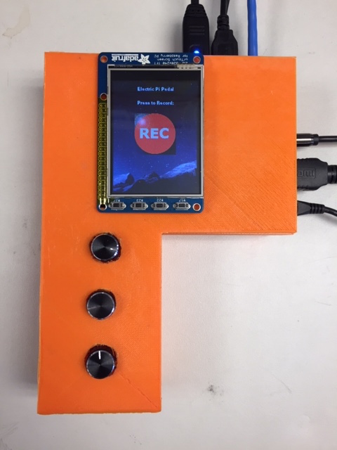
To house the pedal unit itself, we modeled a project enclosure box (Figure 2) in SolidWorks and 3D-printed it using
a Monoprice Maker Select V2 printer in the Maker Lab in Phillips Hall. This enclosure allows for space for the three
rotary encoders, access to the Raspberry Pi's terminals, and a platform to hold the PiTFT display.

Figure 2: Project Enclosure for the Effect Pedal
Software Design
Exploration of Real-Time Capabilities
As mentioned above, we originally wanted to implement a system capable of applying effects to audio signals in
real-time. However, after some initial system development, we were unable to implement a real-time system that
could process audio without an excessive amount of latency. Due to this, we settled on a more segmented
framework consisting of separated system actions: recording, effect application, and playback. This framework
motivated the use of the four distinct processes that will be discussed below.
We will further discuss our challenges with implementing a truly real-time system in the Testing Section.
Multi-processing Framework
The entirety of the code and programs used in the effect pedal resides in a single master program called 'effect_box.py.' This master program is structured in a multi-processing framework where individual processes can communicate using shared global variables that are specified in the main function. We identified four distinct processes that would be run within this master program: the pedal's GUI, the audio recording process, the audio playback process, and the effect-applying process. Furthermore, the global variables shared between these processes all serve one of two purposes, which are either as values representing adjustable effect parameters or as flags representing when to run certain sections of the program.
The global "effect parameter" variables are shared between only the GUI process and the effect-applying process. When the pedal is in use, the user selects the values of effect parameters via the GUI and rotary encoders. The global variables of these parameters are then updated to match the user's selection. When the effect-applying process later accesses the values of these effect parameters, the parameter values match the desired values specified by the user in the GUI.
The global "flag" variables are shared between all four processes and determine which sections of the code to
run. The first of these flag variables that we implemented is a flag that determines whether the entire
program should be running, named "Code_running." When this flag is set to 1, all of the four processes continue
to run. When this flag is set to 0, the four processes all quit. Another flag variable we implemented is a flag
that corresponds to the type of effect that the user picked to modify the audio. Flags like these are used
throughout the multi-processing framework to allow the individual processes to communicate with each other.
Effects GUI Process
Our Effects GUI process was responsible for controlling the system's user interface. We decided to organize our GUI into a series of system screens that would be displayed on the PiTFT. User input (presses on the touchscreen) would allow the user to transition between the different screens and prompt the system to perform different actions. We used PyGame, which we gained experience with in previous lab assignments, to animate the system screens. A python dictionary was made for each system screen, and the value of a state variable determined which dictionary was used to animate the PiTFT screen. Figure 3 shows the state diagram we developed to control the screen transitions.
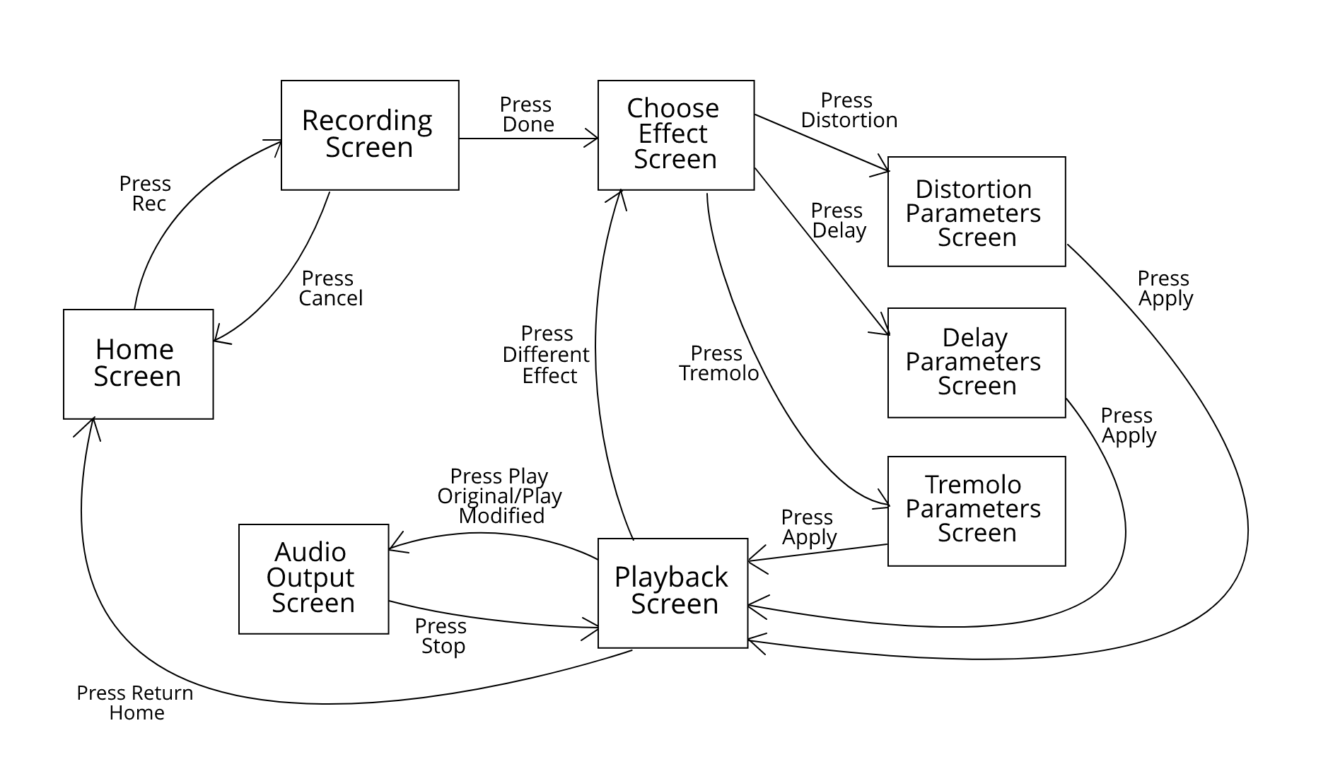
Figure 3: State Diagram for Screen Transitions
Upon startup, the system began at the Home screen. Here, the user was prompted to press a large "REC" button when he or she wanted to start recording audio input. When the user pressed the "REC" button, the Record WAV process began recording audio input, and the system transitioned to the Recording Screen. Figure 4 shows an image of the Home screen.
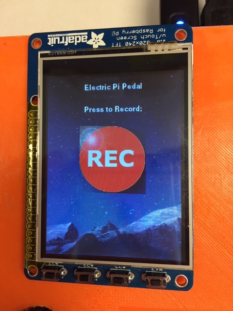
Figure 4: Image of Home Screen
On the Recording screen, the user had two options. The first was to press "Done," which would prompt the Record WAV process to stop and save the recording. Additionally, this would cause the system to transition to the Choose Effect screen. The second option was to press "Cancel," which would delete anything recorded by the Record WAV process and prompt the system to transition back to the Home screen. We felt this would be useful if the user was ever unhappy with the recording. Figure 5 shows an image of the Recording screen.
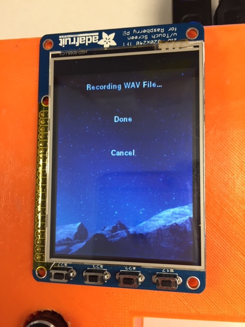
Figure 5: Image of Recording Screen
From the Choose Effect screen, the user could pick an effect to apply to his or her recording. He or she could choose any of the three effects we were able to implement: distortion, delay, or tremolo. When "Distortion" was pressed, the system transitioned to the Distortion Parameters screen. When "Delay" was pressed, the system transitioned to the Delay Parameters screen. When "Tremolo" was pressed, the system transitioned to the Tremolo Parameters screen. Figure 6 shows an image of the Choose Effect screen.
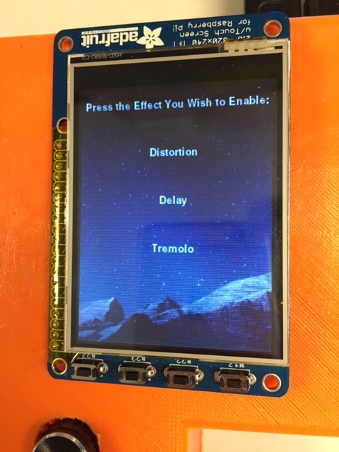
Figure 6: Image of Choose Effect Screen
Depending on which effect was chosen on the Choose Effect screen, the system then transitioned to one of the three effect parameter screens. On these screens, the user could see the current value of the parameter(s) for the chosen effect. By rotating the rotary encoders, the user could change parameter values, and the screen would update to the current parameter values. Inside the Effect GUI process, we defined three GPIO events, one for each rotary encoder. When a rotation was detected, one of the GPIO events would use a callback function to determine whether the rotation was clockwise or counterclockwise. If the rotation was clockwise, the corresponding parameter would be incremented. If the rotation was counterclockwise, the corresponding parameter would be decremented. Once the user was happy with the parameter value(s), he or she could press "Apply" on the screen, which would prompt the Apply Effects process to apply the correct effect to the recording. Additionally, the system would transition to the Playback screen. Figure 7 shows an image of the Delay Parameters screen.
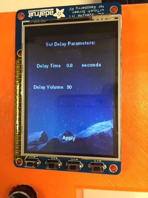
Figure 7: Image of Delay Parameters Screen
On the Playback screen, the user had four options. The first was to press "Play Original," which triggered the Audio Playback process to begin playing the original, unmodified recording. In addition, the system transitioned to the Audio Output screen. The second option was to press "Play New Version," which prompted the Audio Playback process to begin playing the modified recording. In this case, the system would also transition to the Audio Output screen. The third option was to press "Different Effect," which caused the system to transition back to the Choose Effect screen. This functionality was useful when the user wanted to apply a different effect to the recording, after already hearing the recording with another effect applied. Applying a different effect would delete the previous modified recording and replace it with a new one. The fourth option was to press "Return Home," which prompted the system to transition back to the Home screen. This functionality was necessary when the user was finished with one recording and wanted to start a new one. Re-recording would delete the original recording and replace it. Figure 8 shows an image of the Playback screen.
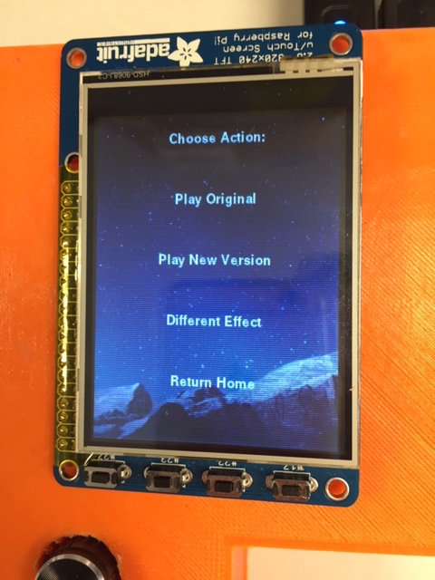
Figure 8: Image of Playback Screen
On the Audio Output screen, the user was able to hear either of the recordings being played back by the Audio Playback process. When the end of the recording was reached, the Audio Playback process would loop back to the beginning and continue playing. If the user pressed "Stop," the Audio Playback process would cease playing the recording, and the system transitioned back to the Playback Screen. This made it easy for the user to compare the recordings by playing one recording, pressing "Stop," and immediately playing the other recording. Figure 9 shows an image of the Audio Output screen.
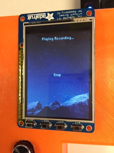
Figure 9: Image of Audio Output Screen
Record WAV Process
The audio recording process begins immediately along with the other three processes in the main function. First, this process globalizes certain constant audio stream parameters set in the beginning of the effects_box.py master program. Next, it opens an instance of PyAudio and sets up a stream to record the .wav file, using the constant parameters that were just previously globalized (these parameters include the format, sample rate, number of channels, input device index, and chunk size). Finally, an empty array named 'frames' is created. This will be used later to store individual frames of the recorded audio.
Once these parameters have been initialized once, the audio recording process idles, waiting for the global record_flag variable to be set high. When the user presses the big red "REC" button on the home screen, this record_flag variable is set high, allowing the audio recording process to enter into the actual audio recording functionality.
Once this occurs, audio input is continually read in through the open stream at the specified chunk size, at which point it is appended to the 'frames' array. This process continues until the user quits recording from the GUI and the global record_flag variable is set low. Next, the array of frames is saved to a .wav file named 'original.wav.' Afterwards, the .wav file is closed and the 'frames' array is emptied. The audio recording process then returns, waiting for the record_flag variable to be set high to record again.
Apply Effects Process
The apply effects process also begins immediately upon startup, where it first globalizes the same set of audio parameters used in the previous process. These parameters are used later in the program to save the modified .wav file in the same desired format. Next, the process specifies certain constants used in calculating each individual effect. The first effect constants are used in mapping the value of the global distortion parameter to the maximum value of the distortion threshold itself. The sample rate is then specified for use in the delay effect, where it is used in relating the delay time from seconds to frames. Finally, the global delay volume parameter is then mapped to a maximum set value.
The functions that calculate and apply each of the audio effects are then defined. Each of these functions accepts the audio file itself, written as an array of 16-bit signed integers, stored in 'signal.' These effect functions also accept certain parameters which ultimately correspond to the global effect parameter values chosen in the GUI.
The distortion calculation function parses through the array of signed 16-bit integers. If any values exceed the threshold specified by the threshold_param parameter, they are clipped and set to that threshold parameter. If the values do not exceed this threshold, they are left alone.
The delay calculation function essentially adds early frame values to later frame values. The number of frames between each frame value and when it is later added is contingent on the delay_time_param parameter. This corresponds to the time it takes to hear the echoed delay. Before the echoed frame is added onto a later frame, its volume is diminished from anywhere between 0% and 100% its original value. This decrease in volume is determined by the delay_volume_param parameter.
The tremolo calculation function splits up the array of 16 bit integers into chunks of a set length that corresponds to the tremolo_speed_param parameter. It then diminishes the volume of every other chunk by between 0% and 100% its original value. This decrease in volume is determined by the tremolo_intensity_param parameter.
Next, the apply_effects process waits for the global apply_flag variable to be set high before continuing. Once the user decides to apply an effect to the .wav file, the process calculates the aforementioned parameters. These parameters cannot be calculated earlier in the program, since they incorporate global variables shared in the multi-processing system. The process then opens up the orignal, unmodified .wav file, which is named 'original.wav.' The data in this file are converted to an array of signed 16-bit integers, named 'signal.' The apply effects process then identifies which effect function to apply to 'signal' by checking the value of the global effect_flag parameter. The new signal is then calculated using the previously defined functions and effect parameters.
Finally, the process converts the modified array of signed 16-bit integers into a .wav file. This uses the audio format parameters previously globalized at the beginning of the process, and then saves the new, modified .wav file as 'modified.wav.' The instance of PyAudio is then terminated, and the apply_flag value is set back to zero.
Audio Playback Process
The audio playback process begins at startup, and immediately defines a callback function. This callback function is used to read a single individual frame of the specified .wav file and return its value. After defining this function, the process waits for the global playback_flag value to be set high. Once this occurs, the process then checks which .wav file to play by accessing the value of the global version_flag parameter. The process then opens up the .wav file that corresponds to that parameter (either the original or modified version). Next, an instance of PyAudio is created, and an output stream is defined with the same format, channel, sample rate, etc. parameters of the .wav file. The stream is then started. For each frame of the .wav file, the previously mentioned callback function reads and returns the frame data necessary to play the audio file. The audio file plays continuously for as long as the global playback_flag value is high. Once this parameter is set low, the stream closes and the instance of PyAudio terminates.
Testing
We began this project with the idea of creating a guitar effect pedal that could read a live audio signal, perform the necessary calculations to achieve the desired effect, modify the actual audio signal, and then output the modified audio signal in real time. Our first attempt to do this involved using Python and PyAudio to simply read the audio coming into the Raspberry Pi and then export it live through the DAC. We opened up the stream and successfully conveyed the guitar's audio output through the Raspberry Pi and into an amp with an estimated latency of ~200ms.
In order to cut down on latency, we rewrote the functionality of this process by using C code with the Synthesis ToolKit (STK), which is a collection of open source software for audio signal processing. We successfully replicated this process and found our latency to be much lower, estimated to be around ~50ms. Our next goal was to implement a simple effect that would bitshift the audio signal by 3 places, effectively decreasing the audio signal's volume in real time. However, the STK platform is very difficult to adjust and rewrite. The code flow between reading and then exporting a live audio stream does not allow for a clean way to modify and save the audio signal. With the time constraints for this project in mind, we decided to abandon the idea of using the faster C code in favor the relative ease with Python's slower interpretive code.
We returned to our original Python code and wrote an effect that would bitshift the audio signal by 3 places before exporting it to be played back in real time. This volume decreasing effect was chosen first, since it utilizes the fastest calculation out of any of our potential effects. When we attempted to run this program, the operation failed due to an overflow of the input signal and an underflow of the output signal. The Python program was just too slow to read the live audio input, perform the volume bitshifting calculations, and then play it back in real time. We then increased the size of the input and output buffer, hoping to avoid input/output overflow errors at the cost of a higher latency. This too failed immediately. Slow to give up hope, we then attempted improve the overall processing speed of the process itself by highly prioritizing our audio program in our Raspberry Pi's process scheduler and then devoting an entire core to it. Again, the input overflow and output underflow were too much for the program to be able to run successfully in real time.
While we were disappointed in the lack of real time signal process capability with Python, we saw an opportunity to create a unique looper effects pedal. Looper effect pedals are used by guitarists to record an audio signal with a short length, clip it, and then play it back on a loop. This provides the guitarist an instantly-made backing track to play over. We decided to restructure the design of our effect pedal to act as a looper effect pedal that had a unique capability to add implement effects to the looped audio. This solution allowed us to retain a real-life functional use case for the pedal and add custom effects to the guitar's audio, all with the convenience of Python.
Results
The video of our final demonstration can be seen here.
As we stated earlier, we were able to implement three effects on our system: distortion, delay, and tremolo.
While we would have liked to implement a few more, the difficulties discussed in the Testing section prevented
us from having the time to do so. With that said, we are still satisfied with the effects we had time to finish.
Figures 10-13 show waveforms for a pure A-440 sine wave and the impact each effect had on that sine wave.
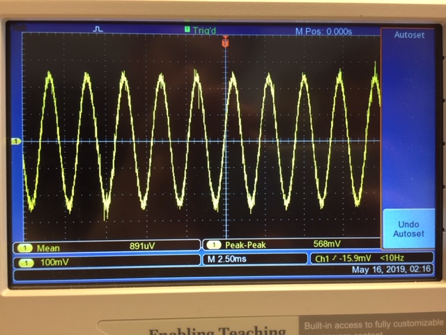
Figure 10: Pure A-440 Sine Wave
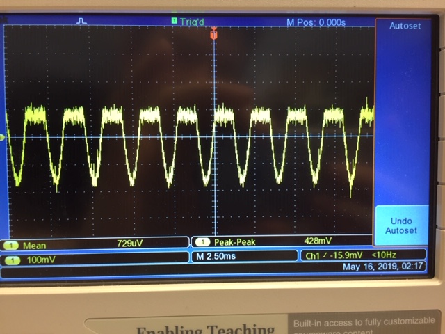
Figure 11: A-440 Sine Wave with Distortion Applied
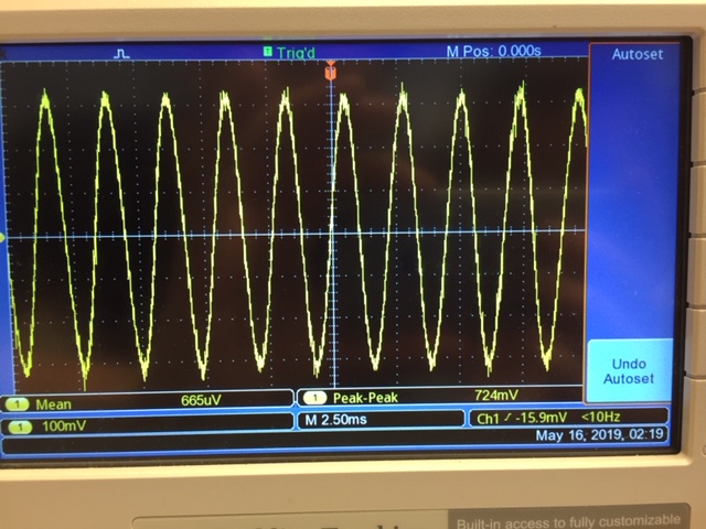
Figure 12: A-440 Sine Wave with Delay Applied
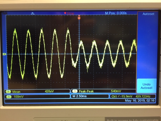
Figure 13: A-440 Sine Wave with Tremolo Applied
In Figure 11, the positive peaks of the sine wave have been cut off. This represents the "hard-clipping" that is
the signature indicator of a distortion or overdrive effect. The amplitude at which the "clipping" begins was
controlled by the threshold parameter.
In Figure 12, it is not so obvious that a delay effect is being applied. However, by comparing the waveform in
Figure 12 to the waveform in Figure 10, we can see that the waveform in Figure 12 has a greater amplitude. This
is caused by the delayed signal being overlayed on top of the original signal and increasing the overall signal
amplitude. Hence, although it is not obvious, the delay is present.
In Figure 13, we can clearly visualize the volume variations because the two neighboring sections of the waveform
clearly have different amplitudes. If we were to zoom out, we would see many alternations between the higher
amplitude and lower amplitude sections.
In terms of the user interface, we were able to successfully implement all of the functionality discussed in the
Software Design section. We were able to get clean transitions between all of the different system screens, as can
be seen in the demonstration video.
We were also satisfied with the audio quality we were able to achieve with our system. We chose a very standard
sample rate of 44.1 kHz for our audio processing. Due to the limitations of the 1/4" guitar jack to USB cable we
used, we chose a bit depth of 16 bits. We were a little worried that this bit depth was going to be insufficient
and would have preferred to use 24 or 32 bits. However, we felt that our system's final audio output had adequate
quality.
Conclusions
After redesigning the effect pedal to function as a looper pedal with built-in effects, the program ran completely as intended. We incorporated a multi-processing framework to keep track of globally used adjustable parameters and flags between various processes of the effect pedal. This multi-processing framework was slightly annoying to implement at first, but it ended up solving the communication issues between our individual processes. The sounds produced by our effect algorithms are easily discernible in our project video, and they match our expectations of what the effects should sound like. Additionally, the oscilloscope screen captures of how each effect modifies a pure sine wave audio signal matched our predictions of what each shape should look like.
To reiterate our experience with real-time processing on a Raspberry Pi: Python seems sufficient to receive and output an audio signal with relatively low latency. However, we found that it does not succeed in simple real-time modification of a digital audio signal. C code shows a promising ability to succeed in real-time modification of a digital signal, although doing this is difficult and relatively undocumented territory.
Future Work
Given more time to work on this project, we would have liked to expand our number of included effects to include other popular guitar effects like chorus, phaser, and wah-wah. With the very customizable nature of the Raspberry Pi, we also would have enjoyed finding other creative ways to produce our own never-heard-before effects. Even the typical "button and knob" interface seemingly ubiquitous to all modern guitar pedals could be completely reimagined by incorporating unique sensors and display systems.
Code Appendix
Our complete, commented code can be found here.
Budget
We were given a total budget of $100 for this project. The following list shows the budgeted parts we needed for our system:
- Guitar Jack to USB Adapter: $27.09
- Rotary Encoders (5-pack): $10.15
- Rotary Encoder Knobs (10-pack): $7.08
- 3.5mm to 1/4" Adapter: $6.59
In addition to the budgeted parts, we used the following borrowed/unbudgeted parts in our system:
- Raspberry Pi Model 3
- 2.8" PiTFT Touchscreen Display
- 5V Power Supply
- 16 GB microSD Card
- 40-pin Ribbon Cable
- Breadboard
- Various Wire/Resistors
- PLA Filament (for the enclosure)
Adding our budgeted costs together, we had a final system cost of $50.91, which was well below the $100 limit.
Work Distribution
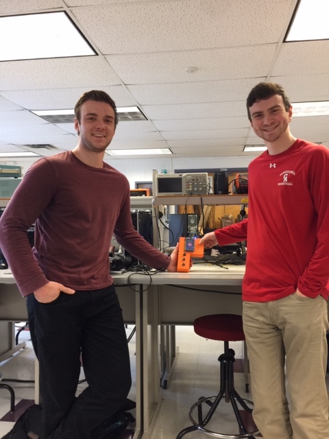
Christian Ray (left) and Ben Roberge (right)
The following lists show the tasks carried out by each group member for this project:
Christian Ray
- Effect Pedal CAD
- Effect Algorithms
- Multi-Process Management
- Rotary Encoder Functionality
- GUI Images
- Lots of Python coding
- Lots of Writing for Webpage
- Guitar Mastery
Ben Roberge
- Effect Algorithm Research
- Lots of Python Coding
- Wired Rotary Encoder Circuits
- Helped 3D Print Enclosure
- Lots of Writing for Webpage