AI Air Hockey
Automated Air Hockey Opponent
Kyle Betts (kcb82), Tharun Iyer (tji8), and Alex Koenigsberger (ak826)
Demonstration Video
Project Objective
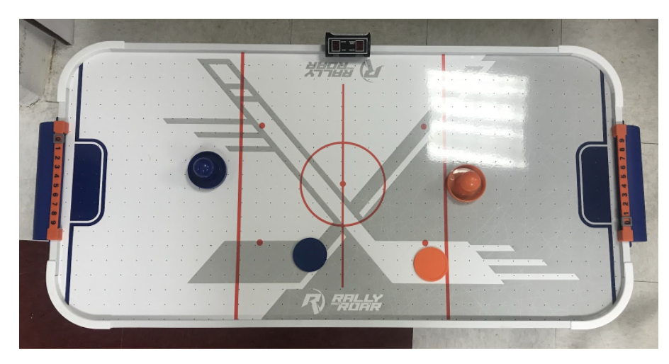
In our project we designed, assembled, and tested an automated air hockey table. Our goal was to have one of the players in the traditional air hockey game be controlled by motors, and the other player be a human competing against the “robot” player. We wanted the movement of the robot player to be educated and strategic decisions based on the position and movement of the puck. While we all enjoy playing air hockey, the issue with the game is that it always requires having another person with you to play it. For only children, people without many friends, or people being isolated due to COVID, this creates a huge restriction in the ability to play air hockey. With our automated air hockey table we solve this problem, allowing people to enjoy the fun game even if they are all alone. At the heart of our system is a Raspberry Pi 4, which does everything from touchscreen UI and motor control to object tracking and strategic planning. We started with a normal air hockey table and finished with a robot opponent able to play against a human on the same table.
Introduction
Completion of the project consisted of three main tasks: assembly of the table, wiring of the electronics and design of the software.
Table Assembly
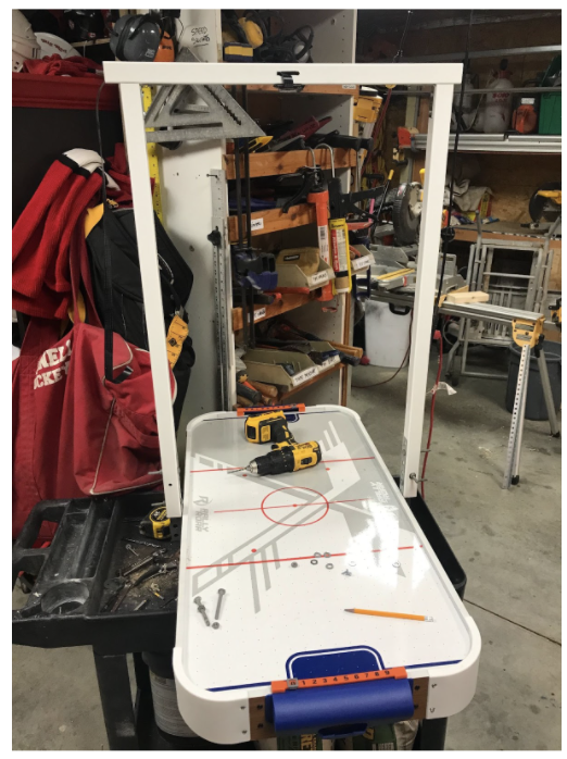
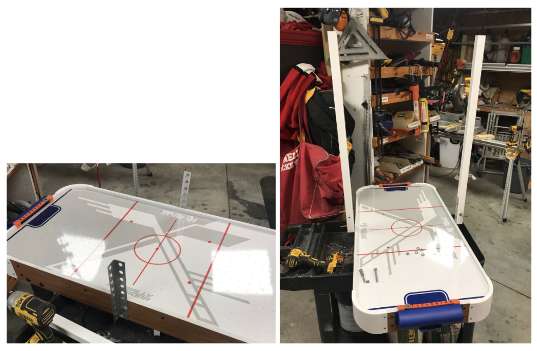
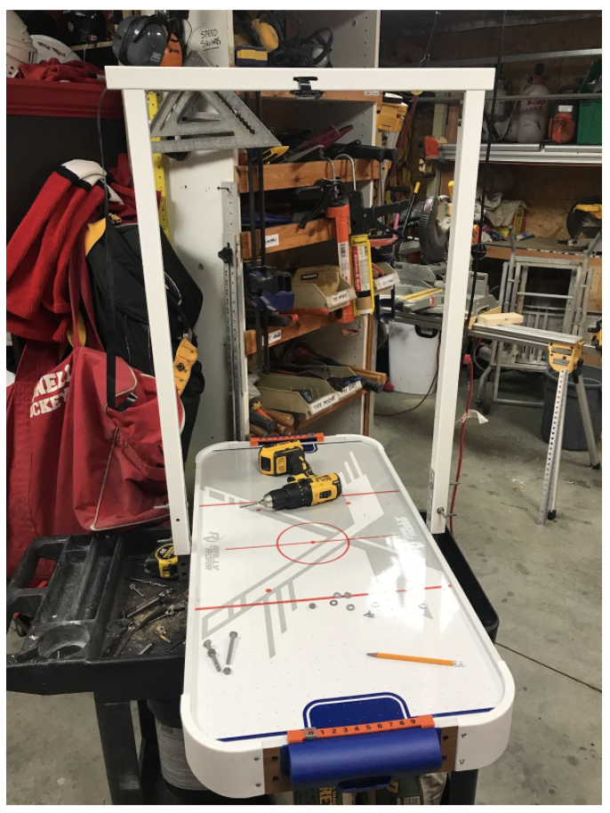
The assembly of the table consisted of a few tasks. The first task was to create a structure above the table for the camera to mount to. This structure had to be high enough above the table for the camera to see the entire playing surface, but also not obstruct the view of the camera and player. We ended up creating a structure consisting of two vertical supports attached on either side of center ice and a horizontal support attached to the top of the two vertical ones to hold the camera.
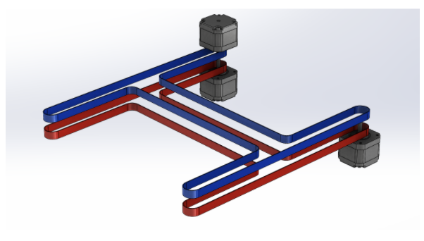
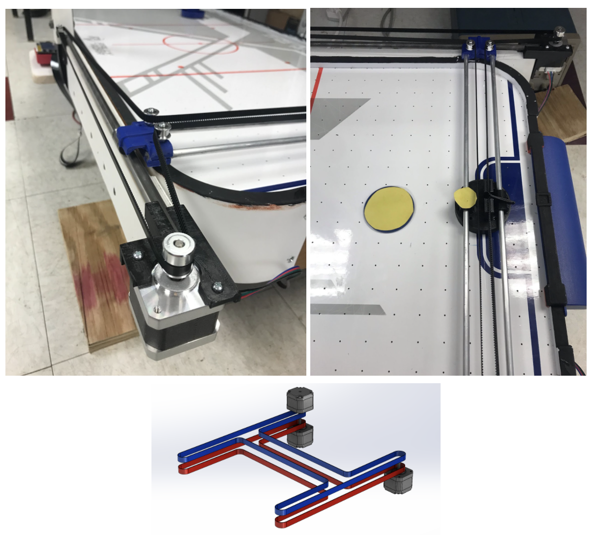
Secondly, the movement system for the robot had to be mounted onto the table. We wanted the robot to be able to move to any location on its half of the playing surface, so this required the movement system to be able to move the robot left/right as well as forward/back. We got our inspiration from the HBot systems sometimes found in 3D printers. With two stepper motors, 6 pulleys and a timing belt, you can quickly and precisely move the robot in any direction required.
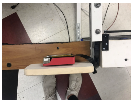
Finally, we wanted the Raspberry Pi to mount to the side of the table near the player's end so that it could be used as a UI to control the game. We ended up mounting a platform off the side for the Pi to sit on, and drilling a large slit into the side of the table for cables to pass through and remain hidden.
Electronics
For the actual connection of all the electronics, the largest and most difficult task came from the control of the stepper motors. Each motor required its own motor controller, and it took us quite a bit of time to figure out how to connect everything correctly to make it work. Outside of the wiring for the motors, the Pi Camera simply connected via ribbon cable directly into the Raspberry Pi, and the PiTFT also connected directly on top of the GPIO pins of the Raspberry Pi.
Software
For the software aspect for our project, we created four separate python programs that run concurrently and communicate
with each other. By spreading the computation over four programs, we were able to utilize all four cores on the Raspberry
Pi and achieve greater performance. Programs are able to start the other programs, with the creating process being called
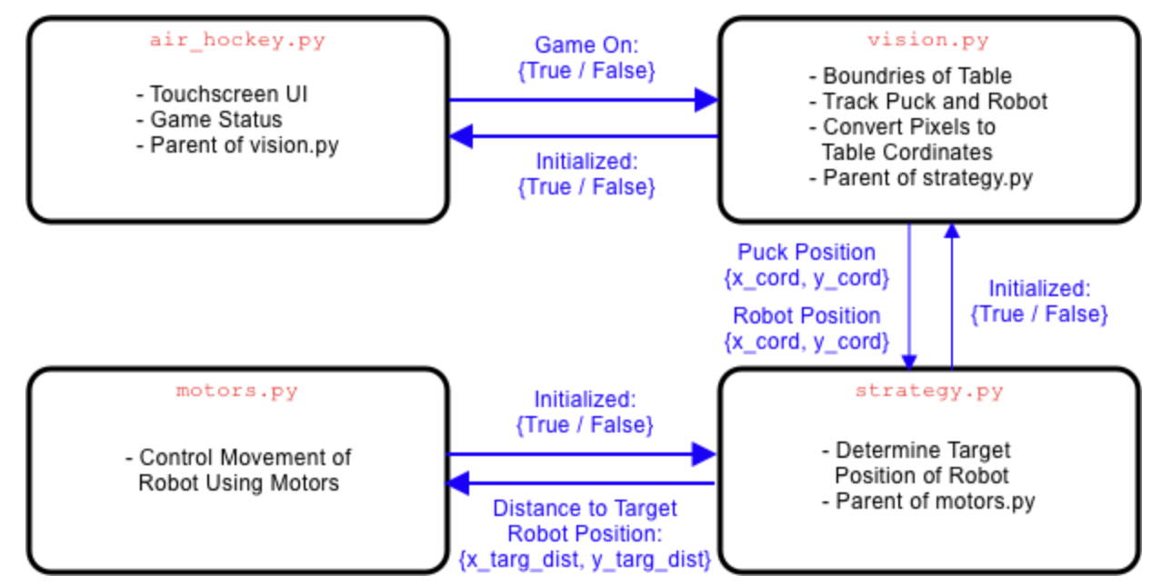
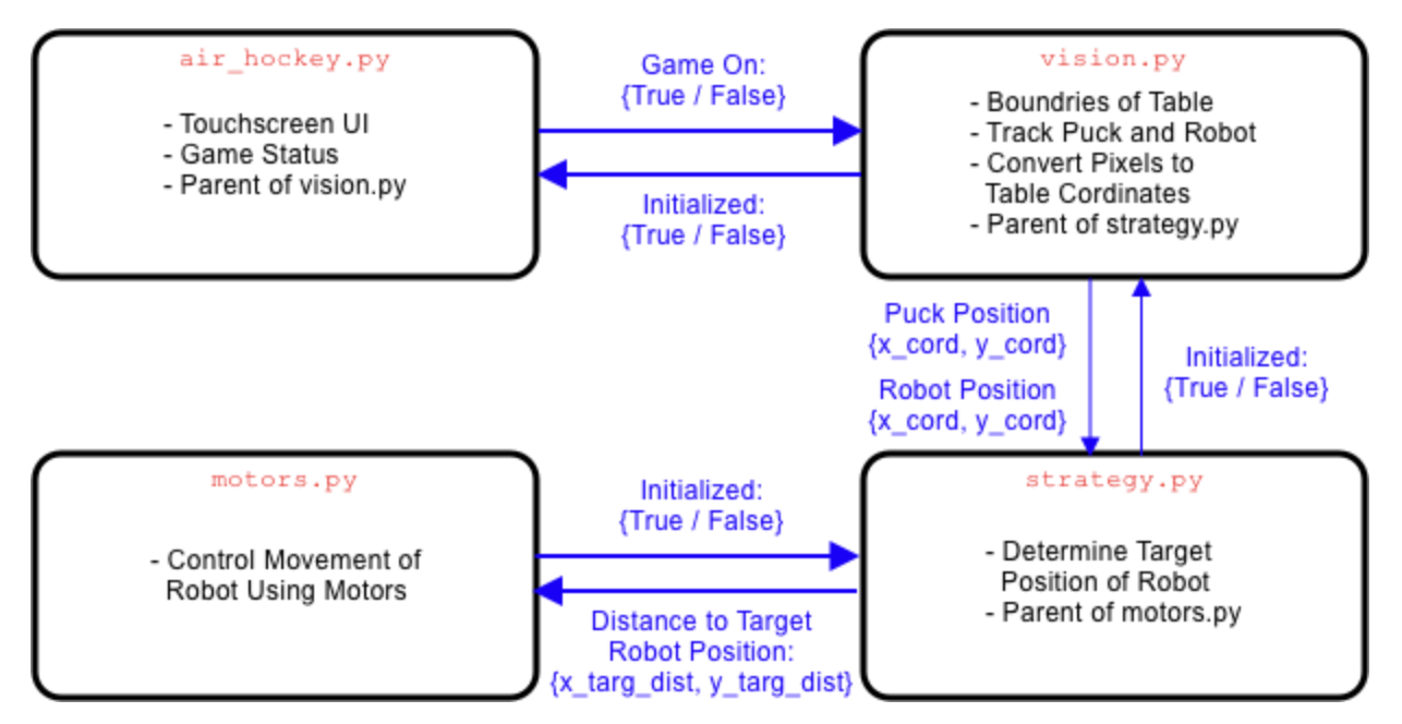
the parent, and the process starting being called the child.The main program, and entry point to the entire system is
air_hockey.py. Its main responsibility is updating the touch screen UI and game status. Its child process
vision.py receives updates on the game status from air_hockey.py, and when a game is in progress, it is responsible for finding
the boundaries of the table, tracking the pixel location of the puck and robot, and finally converting those locations
to table coordinates. The child process of vision.py is strategy.py. The process strategy.py receives the table
coordinates of the puck and robot, and then based on the position and trajectory of the puck strategically decides
where it thinks the robot should move to. The final process is motors.py and it receives the distance to the desired
robot position from its parent process strategy.py. Based on where the robot needs to head, the process sets
the correct
outputs to the motors.
Design and Implementation
Table Assembly
Overhead Structure
The overhead structure serves the purpose of mounting the camera above the table, and also is designed to hide cables running down the structure. We ultimately chose to use some decking railing posts.
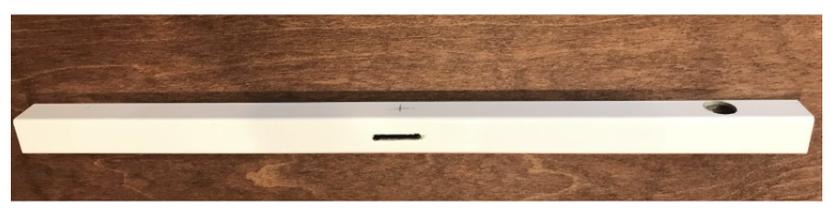
The benefit of using these posts was that we had them as scrap at our house after the decking was replaced, they have a nice white finish, and they are hollow so wires could be hidden in them creating a clean finish. To determine the height that we needed for the structure we connected the Pi Camera to the RPi and measured the height that the camera could see the entire table if above center ice. This value was 35” so we knew we needed the vertical supports of the overhead structure to be 35” above the playing surface. We first bolted metal L supports to the side of the table for strength, and then mounted the cut to height vertical supports to the metal supports. We then grinded off the bolts since they were sticking out a lot.
Next for the horizontal support across the top of the structure we cut it a little bit wider than the width of the vertical supports to create a nice T appearance at the top. We also mounted the Pi Camera in the middle and drilled a slit in the middle for the ribbon cable to go through and hide. Finally we drilled a hole on the end of the support in line with the vertical support so the ribbon cable could come out of the top support and down the vertical support to where the Raspberry Pi would eventually be mounted.
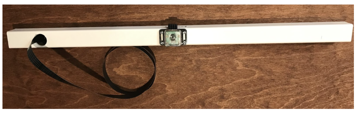
Finally we mounted the horizontal support to the vertical supports using metal L brackets and small screws. The ribbon cable for the Pi Camera was fished down the vertical support as well creating a clean hidden cable system.
Robot Movement System
The first task on the robot movement system was to 3D print the required parts. While we printed our parts in black, ideally you would want to print the parts a color that is common on your playing surface such as white in our case. The parts can be found in our github repo. The breakdown of parts is:| Part Name | Quantity | |
|---|---|---|
| BRUSHING.stl | 2 | |
| LATERAL_SLIDER.stl | 2 | |
| LATERAL_SUPPORT.stl | 2 | |
| MOTOR_SUPPORT_LEFT.stl | 1 | |
| MOTOR_SUPPORT_RIGHT.stl | 1 | |
| ROBOT.stl | 1 |
A major issue we encountered was the parts that were 3D Printed. A lot of stress is put on the parts due to motor vibration, belt movement or due to the ball bearings sliding on the steel rods. Therefore, we had parts breaking because they could not handle the mechanical stress. We printed parts using PLA first at 0.1mm Layer Height and 30% infill. This did not work as the Lateral Support and Slider broke on the first test. In the second iteration, we printed the Lateral Support using ABS and PVA supports and this worked very well. The PVA supports are water soluble and hence dissolve in 3 hours after being placed in warm water. This helps a lot as removing PLA supports may not be easy and sometimes, if not done properly, causes the parts to break. But, the Lateral Slider broke this time too because the layer height and infill were not enough. Ultimately, we were able to solve the issue by printing the parts at 0.15mm layer height and 70% infill using PLA. This made the parts a lot stronger and they could face the mechanical stress. Hence, we recommend printing the parts at the finest layer height and maximum infill possible to decrease the chances of parts breaking.
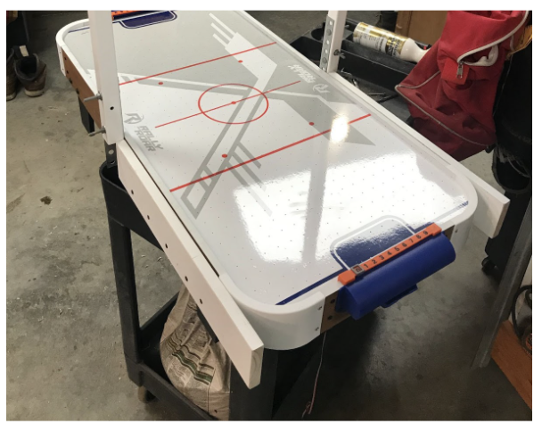
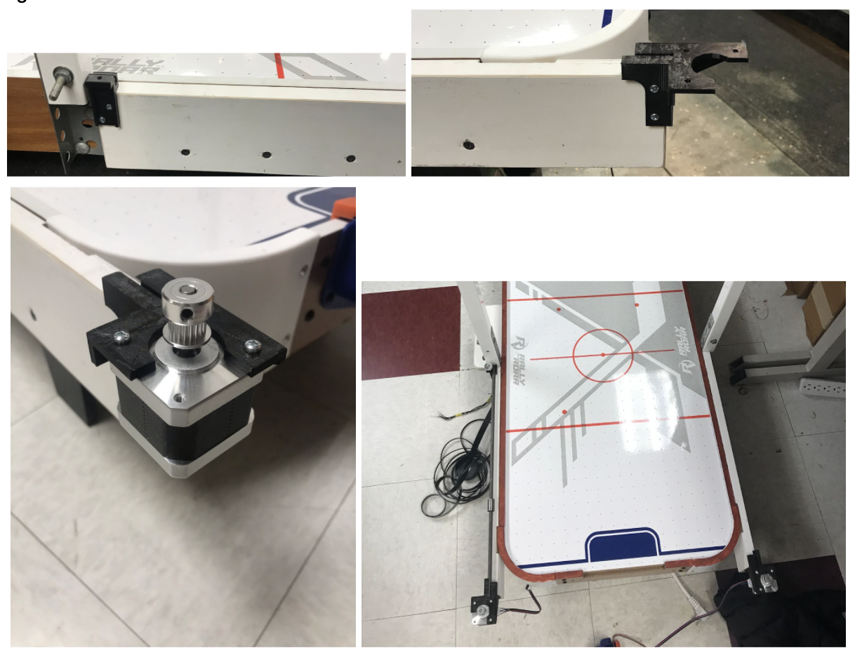
The next problem we encountered is that the motor supports are intended for a square corner to mount to. Our air hockey table has rounded corners so we had to work around this. We did this by extending the edges of our table with some pieces of wood. We extended the walls so that the sides ended a little past the end of the table, which ensured that the robot would be able to move all the way back to its end wall. We simply cut two pieces of wood and screwed them to the sides of the table.
Next it was time to mount the side rails. First we cut two pieces of the steel rod to be the same lengths as the wood we just cut. Then we mounted the lateral support 3D parts to both sides as close to the vertical supports as possible. Then we pushed a linear ball bearing onto each rod, and pushed the rod into the lateral supports. Finally we pushed the motor supports onto their respective side rods, and screwed them into the wood. Finally we attached the motors to the motor supports using 3M bolts, and attached the motor pulley onto the motor shaft and screwed it tight.
At this point the forward/backward rails were complete, and we moved on to the left/right rails. The first thing to do was glue the brushing 3D parts onto the robot 3D part. This is where the rods pass through for the robot left/right track. Next we cut the aluminum rods to the distance between the forward/backward rails. The rods push into one of the lateral sliders, Then the robot slides onto the rods, and finally the other end of the rods is pushed into the other lateral slider. The lateral sliders push down onto the linear ball bearings on the forward/backward rails. Be careful at this step, we broke the lateral sliders a few times pushing too hard. Be gentle! Finally attach two pulleys to the top of each lateral slider, and one pulley to the top of each lateral support.
Almost there! To complete the HBot structure, we need to attach the timing belt. Start by pushing one end into a clip on the robot. Run the belt in an H pattern, eventually ending up back on the other side of the robot. Push the belt into the other clip on the robot and cut off the excess belt. You want the belt to be fairly tight so that there is no slippage on the motors or pulleys.
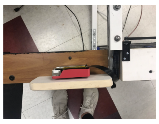
Raspberry Pi Platform
The last part of the table assembly was to create a little platform for the Raspberry Pi to sit on. We cut a rectangular piece of wood slightly larger than the size of the RPi, sanded two of the corners and then screwed it to the side of the table on the player’s side near the vertical overhead support that has the ribbon cable running down it. We also drilled out a slit in the table side so that cables like the breakout cable could be passed through to under the table. Finally we velcroed the RPi to the platform.
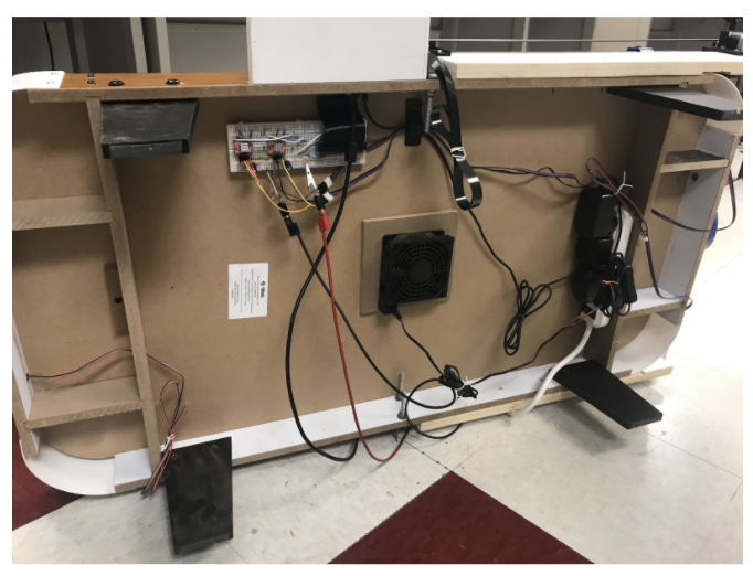
Electronics
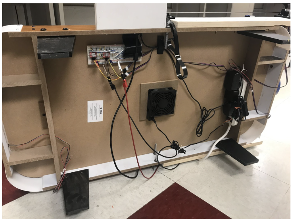
We kept all of our electronics under the table to keep things neat and out of sight. We velcroed a power strip onto the bottom which the air hockey table fan, RPi, and our 12V power supply for the motors plugged into. This allowed us to have a single cord for everything.
Motors
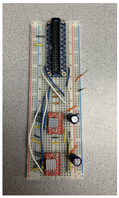
The HBot was controlled with two NEMA 17 stepper motors, each driven with an A4998 stepper driver circuit. The driver has a STEP pin, which causes the motor to step when it goes from low to high, and a DIR pin that sets the direction. It also has pins M1-M3 to set the microstepping mode. The circuit was put together along with the RPi GPIO connector on a single breadboard. On the left rail we had the 3.3V from the RPi connected driving the + rail for our logic high, and GND on the - rail for our logic low. The right rail was reserved for the DC power supply, which we set to 12V to power the motors.The A4998 driver was connected according to the connection guide here, but in summary was connected as follows:
- The active-low ENABLE was pulled to ground.
- The M1, M2, M3 pins, which set the microstepping mode, were connected high, high, low, respectively, to set the motors to ⅛ microstepping mode.
- The active-low RESET and SLEEP pins were shorted together and pulled high.
- The STEP and DIR pins were connected to GPIO pins on the RPi, with a 1k current-limiting resistor in series to protect the pins.
- VMOT and the adjacent GND pins were connected to the positive and negative power supply rails, and they were also connected to a 100µF capacitor to decouple it.
- B2, A2, A1, and B1 were connected to the motor.
- VDD was connected to the 3.3V rail to set the logic high, and the adjacent GND pin was connected to the logic low ground.
The python library RpiMotorLib was discovered, which abstracts away the low-level GPIO control of various types of motors with various drivers. It contains a class for stepper motors with A4998 drivers, which we used to test the motors but ended up too limiting for the final software for the project.
Achieving proper control of our motors, or any kind of control for that matter, was a great challenge to us. The first couple of times that we attempted to build a circuit for an a4998 driver, the motor would either not move at all or it would move erratically even when no program was run to drive the STEP and DIR pins. Even when we adjusted the current control potentiometer on the driver, we would see no change. We are pretty sure we fried the first motor driver that we attempted, as the outputs stopped moving at all when the inputs were stimulated, and had no better luck with the second driver out of the pack of 5.
Exasperated, we switched over to attempting to drive the motor with the TB6612FNG DC motor driver from the Lab 3 robot. One may wonder how a stepper motor can be driven with a DC driver, but it is possible. The motors are simply a certain sequence of outputs that set the voltages on the coils in an order such that the motor rotates. So, with a DC driver, one simply pulls both the PWM pins high and changes the input pattern in the proper sequence to step the motor. Since stepper motors have 4 inputs, one DC driver controls one stepper motor. RPiMotorLib contains a class for driving steppers with this driver, so we tested the motor using the test program included in the library. We found that the stepper motor only turned properly during the “wave” mode tests in the software, which seemed like a victory for us. However, when we inspected the outputs using an oscilloscope, they were extremely noisy and the square wave’s voltage was too low. In addition, the motor pulled a high amount of current, and the supply voltage would drop. Thus, the motor still was not working satisfactorily.
We attempted switching back to the A4998 driver, and it worked after changing out the driver one more time. We are not exactly sure why it did not work the first time, nor do we know why we were unsuccessful with the DC driver, especially seeing how another project group had no issues with driving a stepper motor with the DC driver, however, their motor’s input wires looked slightly different than ours even though it was also a NEMA 17, so that may be the difference. In any case, the motor worked with the A4998 stepper driver and our carefully constructed circuit.
Camera & PiTFT
For the camera, since the ribbon cable was already fished down the overhead structure, we simply plugged the ribbon cable into the RPi’s camera slot. For the PiTFT we ran the breakout cable through the slit in the wall so it could attach to the breadboard under the table. Finally the PiTFT simply pushed onto the GPIO pins of the RPi.
Software
All of our code was written in Python for this project and can be found in our GitHub repo. As shown in the introduction, the purpose and connection between are four processes are:
We needed to use four processes because trying to run all of the logic in one thread would have been too much to ask from one core. vision.py is extremely computationally heavy and if we tried to calculate our strategy (another computational heavy algorithm) in the same thread it would slow down our frame rate of vision.py resulting in poor performance of our robot. When we had all of our code in a single program, our frame rate of our camera was dropping to near 10 FPS, much too slow for robot prediction. Once we split up our program as shown above, we achieved nearly 30 FPS at all times for our camera, a huge improvement.
Interprocess Communication
Since we want to make use of the four cores on the RPi by running four different programs we need a way to communicate between processes. For this we used Python's multiprocessing library and more specifically the Pipe connection object. To use this library, at the top of each file include from multiprocessing import Process, Pipe. Creating a new Pipe returns a pair of connection objects, and the Pipe allows for two-way communication. To create a connection between two processes simply call Pipe(). Now this returns a pair of connection objects, one for the process that made the Pipe() and one for the process it wants to connect with. The creating process needs to send the other connection object to the process it wants to connect to, which we’ll discuss in the next section. As for using the Pipe, we used three simple calls on the connection object: .recv(), .send(object), and .poll(). The .recv() method is used to wait for a new object sent from the other process that the connection is with. This method blocks execution until something is received. The .send(object) method is used to send an object to the other process that the connection is with. The .poll() method returns True if a message is waiting to be read using recv() from the other process that the connection is with and False if no message is waiting to be read. With all of this considered, we are now ready to discuss parallel processing and how it works together with interprocess communication.
Parallel Processing
To implement the parallel processing required to run four processes simultaneously we used Python's multiprocessing library. This library worked exceptionally well and the documentation was easy to understand with great examples. To use this library, at the top of each file include from multiprocessing import Process, Pipe. To illustrate how we used the library I will use an example. Our game begins by calling air_hockey.py which is responsible for launching the vision.py program. To have this work, vision.py must have a function that defines the execution of the program and that function must take a connection object as a parameter. In our case our function is called vision(conn)vision(conn). In air_hockey.py, you must import the function using from vision import vision. Now for the function in air_hockey.py that starts the vision.py program.
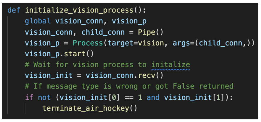
As can be seen, we first have globals for the connection object to vision.py and the actual process object of vision.py. Next, we create a Pipe which gives us two connection objects, one for us and one for vision.py. Next we create a process by specifying the function of the process, and passing that function the other connection object returned by the Pipe(). In this case, we want a process that is the execution function (vision(conn)) from vision.py and we specify which connection object we want to pass to that execution function. Next we call .start() to start the process, which means after this line, vision.py is now also running! You’ll also notice that now air_hockey.py calls .recv() on its connection with vision.py which blocks its execution until it hears back from vision.py saying it’s ready. The first thing we do in the vision(conn) function of vision.py is save the passed connection object as a global variable. Both processes now have their connections to each other saved globally! vision.py now does the initializing things it needs to and once finished it uses .send([1, True]) to inform air_hockey.py that it has finished initializing. First variable in the object is the message type, in this case an initialization response message, and the second variable is True meaning it was successful. Once air_hockey.py receives this message, it is unblocked and returns to normal execution so both processes are running simultaneously!
Startup Process
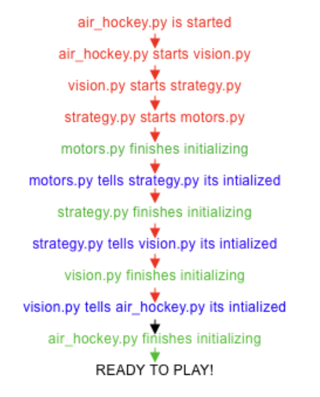
The way our program is set up, each process is at most the child of one process and the parent of at most one process. The way this works it air_hockey.py is responsible for starting vision.py which is responsible for starting strategy.py, which finally is responsible for starting motors.py. This leads to this sequence of events before all processes are ready and the game begins:
air_hockey.py
The air_hockey.py process is responsible for the touchscreen and the game status. It is the main starter program that is the parent of the vision.py process.
The GUI contains a main menu screen with a start and an exit button. The game begins when the start button is pressed, and the entire program exits and subprocesses are terminated when the exit button is pressed. While the game is running, the scores are displayed, but the current version of the project does not include goal detection hardware. There is an exit button that returns to the main menu when pressed.
This process also spawns the vision process and informs it whether or not the game is running.
vision.py
The vision.pyimport cv2 as cv in the python file, and also installed OpenCV on the Pi with the following commands:
As for the actual functionality, once air_hockey.py starts vision.py>, vision.py starts strategy.py and waits for it to finish initializing. vision.py then starts the camera video by calling cap = cv.VideoCapture(0). Next, the program initializes the table. By this, I mean we need to determine what pixels of the video correspond to the walls of the air hockey table. We tried many things to make this work before finding a successful strategy.
First, we tried using Canny Edge Detection (https://docs.opencv.org/4.x/da/d22/tutorial_py_canny.html). This method requires turning an image to grayscale, and then the Canny algorithm uses the greyscale value to determine edges within the photo. The determined edges are left in the image while everything else is filtered out. With the filtered out image we then used contours (https://docs.opencv.org/4.x/d3/d05/tutorial_py_table_of_contents_contours.html) to determine the shapes in the lines. We figured we would be able to look through the shapes and find a rectangle roughly the size of the table we are expecting. While it did a decent job determining edges of the table, it also picked up lots of other edges such as the pattern on the playing surface and shadows. Furthermore, many of the determined edges had missing gaps in them, likely due to variations in the grayscale caused by lighting variations. Ultimately the determined edges were not sufficient to predict the location of the table, so we scrapped this method.
The next method that we tried was Hough Line Transforms (https://docs.opencv.org/4.x/d6/d10/tutorial_py_houghlines.html). This method uses the Canny Edge detection as before, instead of using the contours algorithm it uses the Hough Line Transform algorithm. The Hough Line Transform algorithm takes the filtered out image containing edges found from Canny Edge detection and looks for just lines in the image, not all shapes like contours does. This worked better than contours, and it quite consistently found the lines corresponding to the edges of the table. Unfortunately, since we had rounded corners, the lines of the edges of the table were often cut short on both ends, as the “line” it was calculating stopped at the rounded parts of the table. This gave us inaccurate results for table location, so we could not use this method either.
The final method we tried was using image filtering by grayscale color and then using contours to find the shapes in the filtered image. The code is shown below:
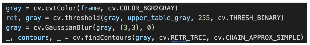
As can be seen, the first step is to convert the image to grayscale. Then you filter out the image based on a maximum threshold of greyscale. 0 is black and 255 is white. The lower you set upper_table_grey, the more is filtered out and darker parts of the image remain. To be able to filter out everything in the image except the walls we painted the walls black. We initially used brown because we had that paint at the time, but the greyscale of brown was too high and got mixed up with shadows. Using black allowed us to set the upper_table_grey to 20 which is very low. Next we used a Gaussian Blur to smooth the filtered image. This helped create a nice smooth border of the table, instead of a blotchy border when not all pixels on the table walls met the threshold. Finally, we used contours to determine the shapes in the filtered and smoothed image. Since all that was really remaining was the outline of the table, the contours typically only contain one shape, which is the edges of the table.
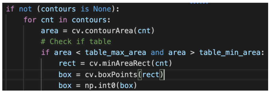
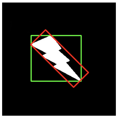
Once we have the contours we do a sanity check. We loop through each shape found in the contours algorithm, and calculate its area. If its area is in the range of expected size of the table, we assume that is the table. Finally, we calculate the minimum containing rectangle of the table's contour. This gives us the smallest rectangle that surrounds the shape and returns the coordinates of the corners of the rectangle. The coordinates of the corners of the rectangle correspond to the coordinates of the corners of our table's walls. In the image below, the red rectangle corresponds to the minimum containing rectangle of the lightning bolt.
Now that the table is located, the initialization of vision.py is complete so it informs air_hockey.py and then it moves onto its main loop. air_hockey.py informs vision.py when a game is on / not on. The main loop pauses when a game is not on, and runs when a game is on. In the main loop there are three main tasks: find the puck and robot, calculate their position in terms of table coordinates, and send these coordinates to strategy.py. To find the pcuk and robot we use hue (color) filtering.
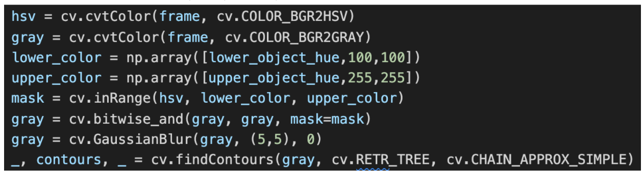
As you can see this is quite similar to the way we detected the edges of the table, but this time we need our image as hsv as well as greyscale. On the hsv image we filter out colors not within the lower_object_hue and upper_object_hue range. For our puck and robot we used yellow paper on them since yellow isn’t anywhere else on our table.
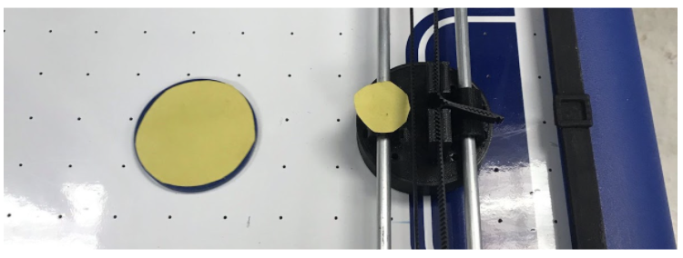
We also tried a dark green but it didn’t work as well. For hue filtering, you want a nice bright color for best results. For yellow our hue range was 20-30. Next we bitwise and the filtered image and the grayscale image. This leaves just the areas that are yellow on the grayscale image. Finally we gaussian blur to smooth the image and find the contours on the masked and smoothed grayscale image. This typically returns just two contours, the larger circle of the puck and the smaller circle of the robot. For sanity checks we still check area ranges as we did for the table contour. The next step is to find the position of the center of the objects, we do this using the minimum enclosing circle.
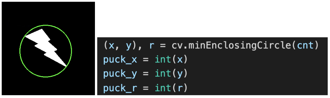
The minimum enclosing circle returns the x and y position of the circle that contains the contour, as well as the radius of that contour. This is shown as the green circle on the lightning bolt contour.
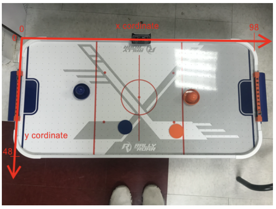
The next part of the main loop is to convert the pixel locations found of the puck and robot to table coordinates. The table height is 48cm and its width is 98cm. We set the coordinates up like below:
To convert pixels to table coordinates you first need a scalar for the pixels per coordinate. This is shown below.

Now to calculate the table coordinate position of a pixel location it is just simple math. The distance:
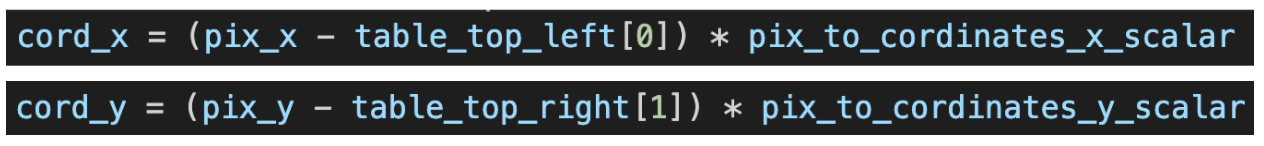
Finally, vision.py sends these coordinates to strategy.py to determine where the robot should go.
The biggest advice I would give would be to have custom lighting in projects using OpenCV which will give you consistent and predictable results. The shadows cast by lab lights, sun coming through windows, and people walking by caused difficulty for us. For the next step, we want to put lights in the overhead structure to make our playing surface illumination more consistent and predictable.
strategy.py
This process receives the location coordinates of the puck and robot from vision.py and uses them to determine the target distance the robot must travel in order to intersect the trajectory of the puck. Since the robot just moves from side to side, the high-level task for this process is to predict the vertical coordinate of the puck when it reaches the horizontal coordinate of the robot. If the puck is moving away from the robot, it tells the robot to return to its center position. The more detailed internals of this process are described as follows.
The position of the puck in the previous frame and its position in the current frame are stored in global variables. The first thing that happens is that the previous position of the puck is overwritten by the values in the current position variables, and then the current position variables receive the values from vision. These two values are then used to approximate the horizontal and vertical velocities of the puck in cm/s by taking the difference and multiplying by the frame rate, which is 30 fps.
With the location and the velocities, the future position of the puck can be estimated. A subroutine called predict_defence_position is entered and the following is done. If the puck’s horizontal velocity is negative, meaning that it is moving away from the robot, the robot target position is set to the center of the positional column that it straddles. If the puck is moving towards the robot, then the future vertical position is predicted as follows:
The slope of the puck’s trajectory is calculated by the tangent of the y- and x-velocities. Then, the predicted y-coordinate of the puck is calculated by multiplying the slope by the horizontal distance between the puck and the robot, and then adding it to the position of the puck.

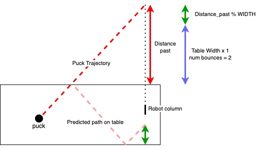
This predicted position, however, is not constrained to be within the table. If it is beyond the width of the table, then it means that the puck will bounce off the wall. We can predict the position of the puck after wall-bounces with the following method, assuming that bounces off the wall are perfect reflections.
- Calculate the distance between the table boundary and the predicted y-coordinate of the puck. We call this
distance_past. - The number of bounces off the wall is determined by 1+floor(
distance_past/TABLE_WIDTH) - The distance away from the wall where the puck will be is equal to
distance_pastmoduloTABLE_WIDTH - The last wall that the puck will bounce off of is determined by the vertical direction of motion and the parity of the number of bounces, and the puck will land past that wall at a distance equal to the value calculated at step 3
Once the predicted position of the puck is calculated, its distance from the current position of the robot is calculated and sent to motors.py. Note that only the direction of the puck’s motion, not its speed, is employed in this prediction. This is because the robot will simply try to get to that position as soon as it can, agnostic to when the puck will actually reach it.
motors.py
This process controls the RPi GPIO pins that drive the motors. It receives the horizontal distance between the robot and the predicted puck location, and from there decides how to proceed.
We had to abandon the RpiMotorLib library because it only has one motor control function, motor_go(), which tells the motor to rotate at a certain frequency for a certain number of steps (and a certain microstepping mode if M1-M3 are connected to GPIO pins). Since this is a python function call, it effectively blocks the process in which it is called until the motor stops moving because the PWM pin is controlled by a loop with time.sleep() calls to set the pulse period and cannot run in the background. We needed much more fine grained and adaptable control of the motor so that it was moving and adjusting constantly and smoothly, so this motor control process was written from scratch. This was very possible and did not take too long a time to implement because the motion of the motor only requires step timing and direction as parameters, and step timing can be done easily in the background using PWM.
The low-level function of the motors are controlled by just a few constructs. The STEP pins are each controlled by a GPIO.PWM instance much like lab 3. However, frequency controls the speed of the motor rather than duty cycle. The duty cycle is set to 50 when the motor is on, and 0 when it is off. The direction of each motor is set with another GPIO pin. As for software variables, both motors’ are controlled by the same frequency variable because they are both always moving at the same speed. There is a maximum and minimum frequency that the speeds are constrained to. This is because the software PWM instance cannot have a frequency of 0, so a minimum frequency must be defined There is also a fixed acceleration value by which the frequency is changed when speeding up or slowing down. This is because it is not good for the motor to change its speed or direction too abruptly, and it also makes the motion of the robot smoother.
The robot can either be speeding up, slowing down, stopped, or remaining the same speed. To set these motions, two functions were written:
speed_up(): Starts the motor back up if it is stopped by setting the duty cycle to 50, and increases its speed, saturating it to the maximum value.slow_down(): Decreases the frequency of the motor, saturating it to the minimum frequency, and clearing the duty cycle if it is at minimum frequency.
One of these two functions is called every time the motor gets a new distance from strategy.py. With this information, it must make a decision on how to move. It was quite easy to simply move left and right in response to the puck’s position by using the acceleration mechanism for smooth motion, but the biggest challenge was to get the motor to stop at its target location using this mechanism. Again, we wanted to avoid abrupt changes to the motor’s direction.
To do this, we needed to find the distance away from the target at which the motor must begin decelerating to a stop. We solved for this using the kinematics formula d=(1/2)at^2 and the fact that time to decelerate to a stop is equal to speed/acceleration. In addition, the target distance was given in centimeters, but the speed was defined by frequency, or motor steps per second, and the acceleration constant was defined in steps per second per update. The steps per centimeter was measured to be 320, and the update rate was approximately 30 per second. So, our final equation for deceleration in centimeters was:
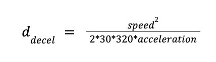
The 30 and 320 in the denominator are the frames per second and steps per centimeter conversion factors. If the motor is within this distance from its target, it should be decelerating.
Every time this process received a message from strategy.py, approximately 30 times per second, it called a function called update_motors() that determined how the motor needed to be moved. The process is illustrated in the diagram below.
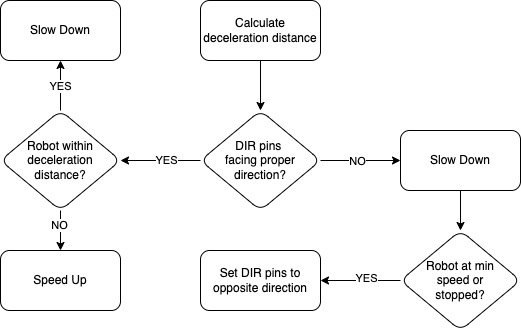
In this way, we control the motors smoothly and adaptively as strategy.py sends target distances.
Results
We successfully constructed a robot that defends an air hockey goal. While originally we were aiming to have the robot moving on both horizontal and vertical axes, we only got up to moving it across the width of the table due to challenges such as troubles with motors and breaking 3D-printed parts. However, this does not mean that this project was unsuccessful because the core of the project, namely the parent process, vision system, game strategy mechanism, and motor control, were all implemented. Any additions to the gameplay would only require modifications to the logic of each of the parts. If the table is slightly inclined so that the puck slides back to the human player if it ends up behind the robot, a single player could be entertained at the table for quite some time. After all, this was the overarching goal - to sustain a game against a fully automated opponent.
Conclusion
This project pushed Raspberry Pi’s capability by incorporating computer vision, I/O control, a touchscreen, and other calculations concurrently in a multi-process system. All of the components were successfully combined to create a limited, but effective automated air hockey opponent.
This project was a great learning experience for all of us, for every group member working extensively on a tool or system in which they had little prior experience. As a result, a number of challenges arose.
As mentioned in an earlier section, successfully controlling the motors was a great challenge. It actually set us back enough to where we were granted a one-day extension for our demo, which ended up being used fully. Nothing that absolutely did not work was discovered here, for every problem we face should have worked in theory. We never could place why our first attempt at using A4998 drivers failed. In addition, driving stepper motors with the lab 3 DC motor drive is certainly possible, for another lab group accomplished this.
Our 3D printed parts broke multiple times due to stress from the mechanism. From this, we learned to not waste time with low quality prints, but rather should jump to sturdier options from the start or after just one low quality print for testing and sizing purposes.
Despite these challenges, we were able to complete what we believe is a successful ECE 5725 project of substantial complexity and great enjoyment.
Future Work
There are a number of additional features that could be added to the project. Firstly, the robot could be improved to move on two axes. This would require the sturdier 3D-printed part to be installed. The strategy process would need to be upgraded to identify scenarios in which the robot could advance from its defensive line and hit the puck back to the player instead of simply blocking goals. Additionally, the motors process would need to enable the motors to move in different directions and different speeds. This would require each motor to have its own frequency variable and the direction control process would likely become far more sophisticated. Since the core of the project is already fully implemented, this would only require software changes to these two processes.
The UI for the project could be improved as well. Currently, there is no score-tracking mechanism but we had originally planned to incorporate one. The air hockey table has built-in laser sensors that we could use, or we could install our own score-detection system and connect it to the RPi, which would then use its input to stop the game whenever a player scores and display the ongoing scores on the PiTFT. Additionally, more “bells and whistles” could be added to the table itself. For example, a string of LEDs could be installed on the camera mount, which would not only include the aesthetic merit of the table, but also help the camera identify features by improving the lighting of the table. For example, a brown outline may become distinguishable from a shadow with better lighting. Perhaps the table could play different sounds during gameplay, such as cheering crowds upon scores, if we incorporated a speaker. Additionally, maybe the scores could be displayed on a 7-segment display or LED matrix that are more visible to the player. There is a lot of room for creativity when considering upgrades to our project.
Work Distribution

Kyle Betts
kcb82@cornell.edu
Actual Hockey Player - Cornell #11, Captain
Built overall structure and helped with HBot
Set up multiprocess architecture and designed vision process
Helped with wall bounce prediction strategy implementation

Tharun Iyer
tji8@cornell.edu
Saw snow for the first time from inside the lab
3D Printing Specialist
Helped construct HBot system and test motor electronics
Built the PiTFT GUI

Alex Koenigsberger
ak826@cornell.edu
Chimesmaster
Tested motors and built final compact breadboard circuit
Designed and wrote motor software
Helped with wall bounce prediction strategy
Parts List
Hardware
| Part | Quantity | Price / Unit | Total Price |
|---|---|---|---|
| 6’ 8MM Diameter Steel Rod | 1 | 6.47 | 6.47 |
| 3’ 8MM Aluminum Rod | 2 | 4.54 | 9.08 |
| LM8UU Linear Ball Bearing | 2 | 0.91 | 1.82 |
| GT2 3mm Bore Toothless Pulley | 1 | 1.40 | 5.60 |
| GT2 3mm Bore 16 Teeth Pulley | 1 | 1.40 | 2.80 |
| 5m GT2 Timing Belt | 1 | 10.99 | 10.99 |
| GT2 5mm Bore 20 Teeth Pulley | 1 | 1.40 | 2.80 |
| Total Cost | 39.56 |
Hardware
| Part | Quantity | Price / Unit | Total Price |
|---|---|---|---|
| Raspberry Pi 4 2GB RAM | 1 | 0.00 | 0.00 |
| PiTFT 2.8” Resistive Touchscreen | 1 | 0.00 | 0.00 |
| 2m Ribbon Cable for Pi Camera | 1 | 5.95 | 5.95 |
| 8 Megapixels Pi Camera | 1 | 29.95 | 29.95 |
| Nema 17 Stepper Motor | 2 | 7.66 | 15.32 |
| A4988 Stepper Motor Driver | 2 | 1.86 | 2.72 |
| 1K Resistor | 4 | 0.01 | 0.04 |
| 100µF Capacitor | 2 | 1.16 | 2.32 |
| Power Bar | 1 | 5.99 | 5.99 |
| Total Cost | 62.29 |
Cumulative
| Hardware Cost | Electronics Cost | Total Cost |
|---|---|---|
| 39.56 | 62.29 | 101.85 |
Code Appendix
All of our code, 3D parts and relevant data sheets can be found in the GitHub repository (https://github.com/kylecbetts/ece5725-final). The folder 3DParts contains the parts that need printed for the project in stl format. The folder Datasheets contains the datasheet for the A4988 motor driver used in the project. Finally, the folder src contains our four python programs used for the project, and an image used on the UI.