Self-Balancing Robot
a ECE 5725 Final Project
by
Alex Lui (al754) and Jordan Brunson (jdb429)
Fall 2018
Introduction
Anyone who’s seen Boston Dynamics videos cannot help but be awestruck (and maybe even a little terrified) of the incredibly graceful and lifelike movement exhibited by their robots. Mobile robots such as these are dynamics and controls masterworks. Drawing inspiration from such great feats as these we thought it be appropriate to try to develop a self-balancing mobile robot. Such a robot, we envisioned, would not only be able to balance itself but also navigate based on user command and do all this while carrying other objects. This, we figured, could be accomplished with a balance control algorithm running on a Raspberry Pi. The balance control would receive orientation data from an accelerometer/gyroscope chip and would issue commands to a motor driver thereby controlling the wheels at the base of the robot. This seemingly straightforward idea would end up becoming a monumental undertaking. Throughout the following page we detail our first ever attempt at creating a self-balancing mobile robot.
Project Objective
The goal of this project is to develop a two-wheeled standing robot that balances itself using its base wheels. This robot should be able to balance while holding an assortment of other objects. Furthermore, it should be able to maneuver forward, backward, left, and right based on a received command. These features will be controlled using a Raspberry Pi.
Design & Testing
The design of the self-balancing robot involved the development, calibration, and troubleshooting of quite a few subsystems and subassemblies (see below list). Despite their coupled nature, each will be discussed individually before elaborating about the system as a whole.
- Robot Frame
- Sensors
- LSM9DS1
- BNO055
- Motor Control
- DC Gearbox Motor
- DRV8833
- Transistor Network
- Additional Hardware
- Control Algorithm
Robot Frame
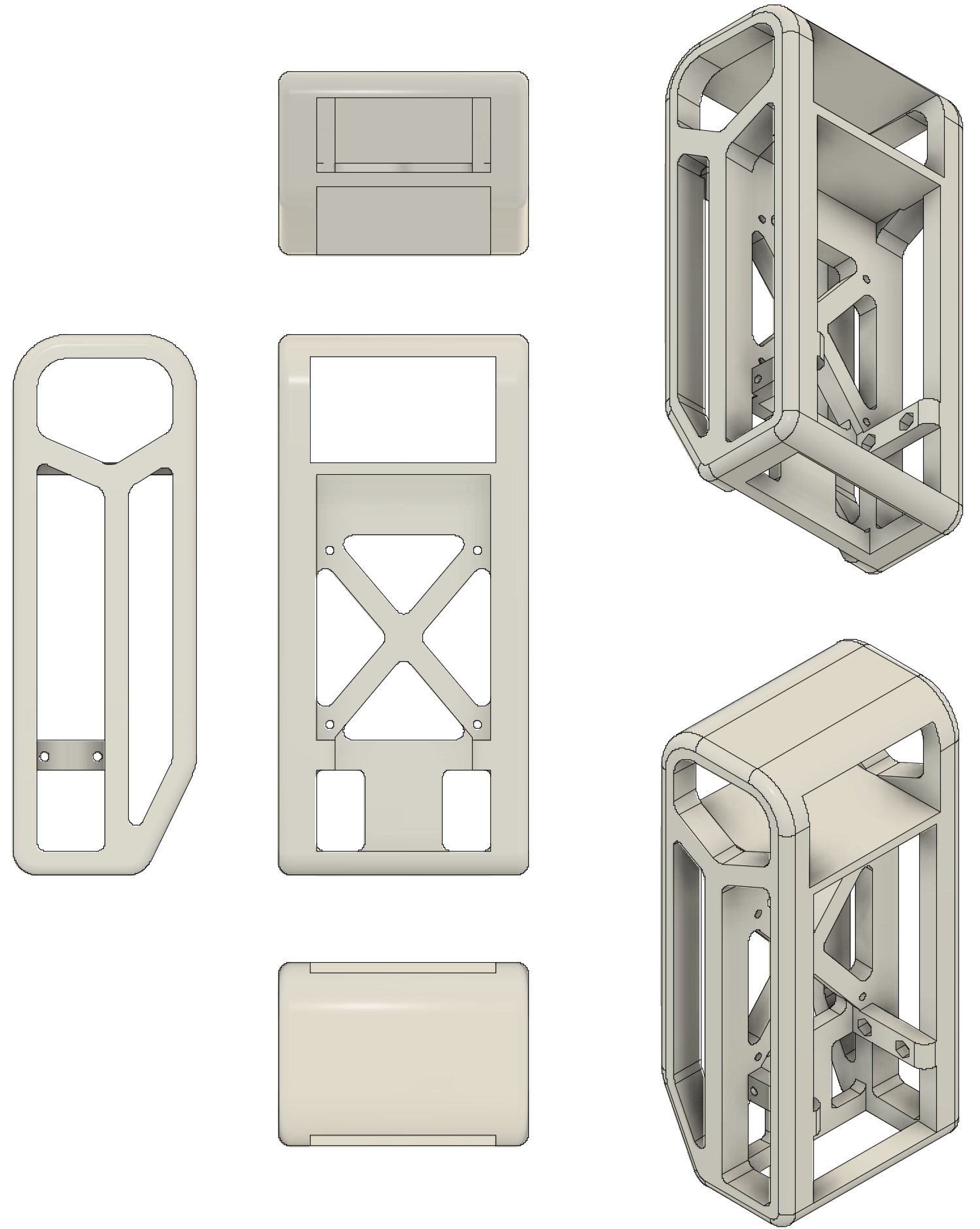
To hold all the components together, a frame had to be developed. The developed frame would have to be rigid while also being accessible. Since we would be using 3D printing, the designs that we would come up with could be complex if needed. One of the initial designs (see below), would have had all the components stowed away compactly in the robot frame.
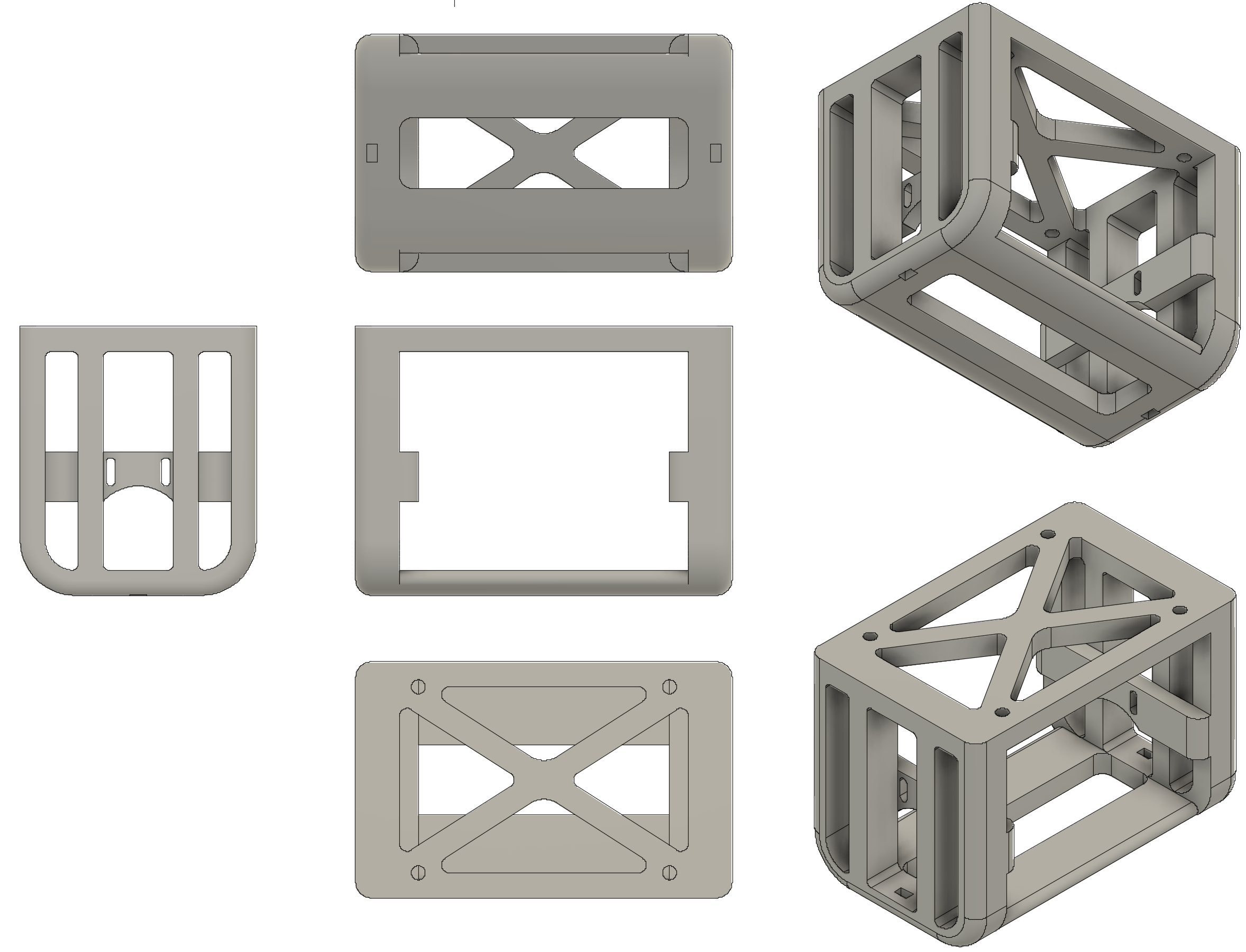
This design ended up being discarded as there was concern over the vertical mounting of all the components and the lack of flexibility in the design. A new design was envisioned that would use a shelf system to hold all the components of the robot. This way the components would be mounted horizontally and, if more space were needed, more shelves could be added (flexibility). The design consisted of a base unit (see below) which would serve as a connection point between the DC motors and the shelf assembly.
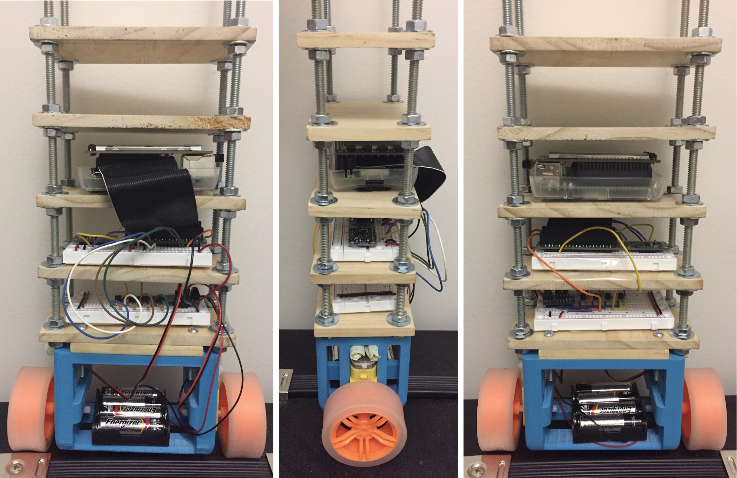
After 3D printing the base unit, a shelf assembly was created using a 0.25” wood sheet and some threaded rod. The robot frame was then fully assembled(see below). At the suggestion of our TA we also installed several "training rods" to the base unit of the robot. These prevented the robot from falling hard on one of its faces. This proved especially useful during the controls tuning phase.
Sensors
Before any balance control algorithms could be developed, a sensor was needed in order to establish the robot’s orientation in space. Determining an orientation requires the use of either an accelerometer, a gyroscope, or a combination of the two. The good news is that accelerometers and gyroscopes are often sold together on the same chip. As it would later turn out, not all accelerometer/gyroscope sensors are equal. This was unfortunately discovered well into our project and led to much frustration.
LSM9DS1
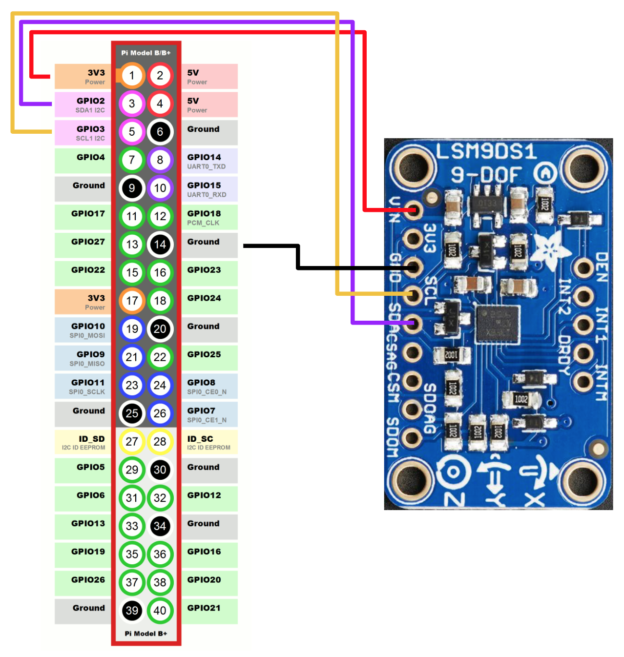
We initially opted to use Adafruit’s LSM9DS1 which contains a 3-axis accelerometer as well as a 3-axis gyroscope. This sensor was particularly appealing due to its relatively lower cost. Once the sensor was received it was wired up (see below) and was mounted to robot frame.
At the time it appeared that the LSM9DS1 prefered to interact with c language as opposed to Python. In order to access the LSM9DS1 data stream, we installed the LSM9DS1 Raspberry Pi Library by SparkFun which, given our best understanding, acts as a Python-c interface (this may not be accurate). As we would find out later, accessing the LSM9DS1 datastream could be done with the Adafruit’s CircuitPython Library.
Fortunately and unfortunately, as our project progressed to its final stages, it was realised that the LSM9DS1 was delivering very noisy data compared to other commercially available accelerometers/gyroscopes. This was understood after countless hours of perplexion over why our robot was so bad at balancing. In addition to the noisiness of the measurements, all accelerometer data received from the sensor was a measurement of the total perceived acceleration. This meant that in addition to the perception of the gravity vector, the accelerometer would also pickup the other accelerations caused by the pendulum swinging motion and the acceleration of the wheel base. Such acceleration measurements cause the balancing algorithm to mistake its true orientation. While it was good that we were able to identify the suboptimal component, it was sad that it happened so late.
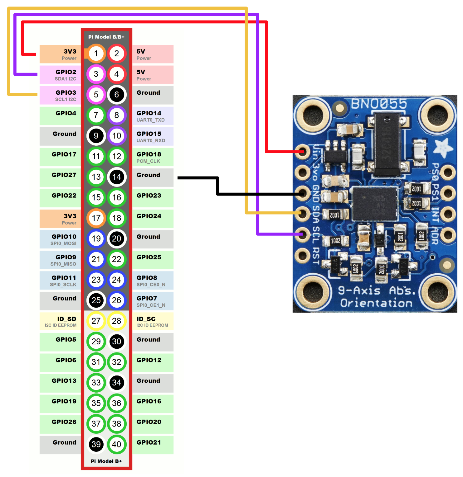
BNO055
In order to combat noisy accelerometer and gyroscope measurements, we acquired the BNO055 from our beloved TA, Xitang. Beyond the cleaner measurements, this sensor has the built in capability of measuring absolute orientation. This was a much welcome feature as it eliminated the need to include acceleration corrections in our balancing algorithm. The only downside to the new sensor was substantially higher cost (more than double the cost of the previous). The BNO055 sensor was wired up (see below) and was mounted similarly onto the frame of the robot.
Motor Control
The mechanism that fundamentally keeps the robot balanced is the actuation of the wheels at the base of the robot (essentially an acceleration to arrest the falling motion). In order to make this happen it was essential to acquire a pair of DC motors and a motor driver. As it turned out, the specific motor driver that we acquired would had certain requirements that hadn’t been carefully considered before hand. This ended up presenting a challenge which caused delay in out project.
DC Gearbox Motor
The specific motor that was chosen for our project came with the recommendation of Professor Skovira. The DC motor selected had a power input range between 3 and 6 VDC. Adafruit measured the motors to spin at 200 RPM and deliver 0.6 Nm of torque at 6 V. In hindsight, this value was probably too low for our robot as this figure only translates to around 35 cm/s. We had selected the motors before constructing the framework, so we did not realize how fast we needed to recover from a falling motion.
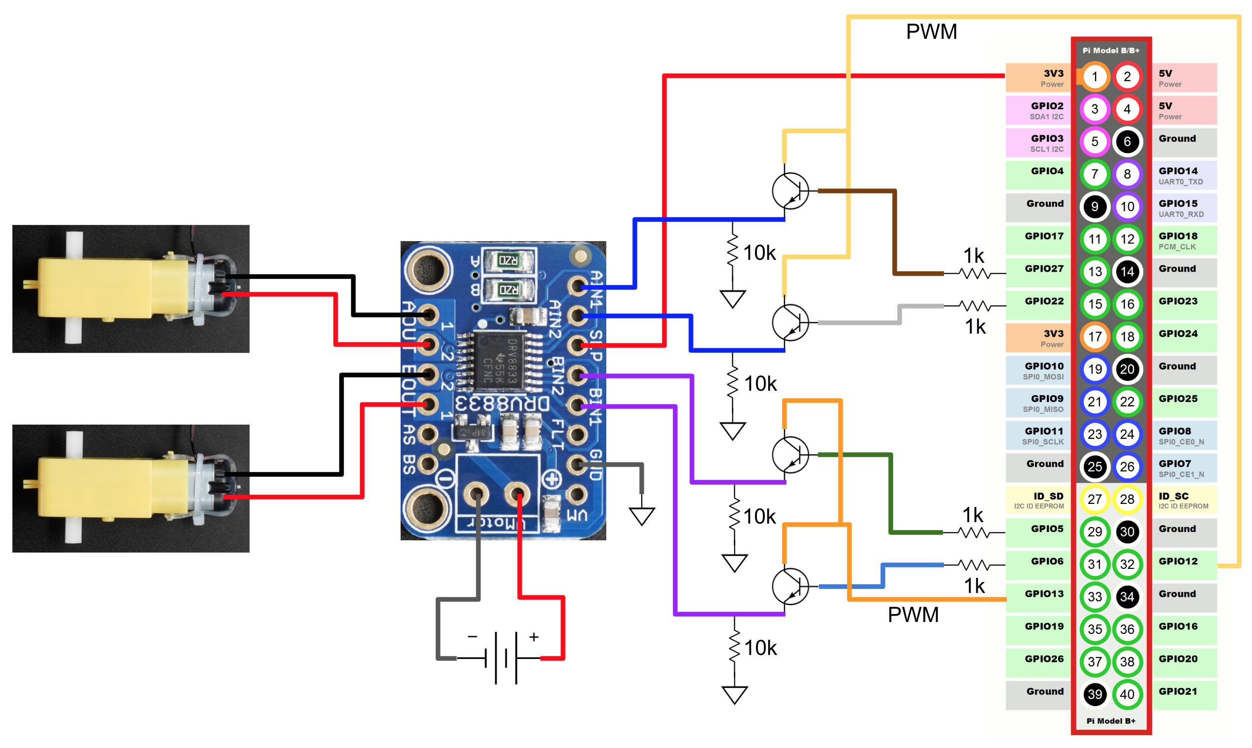
DRV8833
To control our DC motors we had to get a motor driver. We ended up choosing the DRV8833 as it was the Adafruit’s recommended motor driver for the DC Gearbox Motor. The input parameters to the DRV8833 are shown in the following figure:
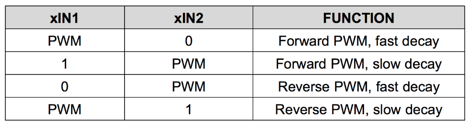
Inside the motor driver are two H-bridges that require two pins each (Ain1 and Ain2 or Bin1 and Bin2) to control the direction of one motor. One pin has to be high while the other has to be low for the motor to spin. Depending on which is high, the motor rotates in a certain direction. Since the robot has to quickly change its speed and direction to balance itself, a PWM signal is required at the “high” pin to control how fast the motor rotated while the low pin’s PWM signal temporarily has a duty cycle of 0.
Based on this input requirement, we needed four PWM signals for the two motors; two would have duty cycles of 0 and the other two would determine how fast the motors spun. However, after a while of testing and debugging, we realized that the Raspberry Pi only has 2 hardware PWM pins! This caused some initial panic as acquiring a new motor driver would take a while. Thankfully, with the help of Professor Skovira, a clever workaround was developed.
Transistor Network
With the help of Professor Skovira, we experimented with switching a PWM signal on and off using a transistor controlled by a GPIO pin. When the GPIO signal is “high”, the PWM signal is transmitted through to the input terminal of the motor driver. If the GPIO signal is “low” the PWM signal is cut off from the motor driver. Using this technique a single PWM signal could be split between two motor driver input terminals by having one active and one inactive transistor. This ended up reducing the number of required hardware PWM pins at the affordable price of four transistor controlling GPIO pins. The following is the final version of our transistor network:
Control Algorithm
The vertical stance of the robot is an unstable equilibrium. Any small deviation from a perfectly vertical stance will cause the robot to swing away from that equilibrium due to the torque generated by gravity. Without any control mechanism in place, the robot will abruptly fall over on its side. To combat this, whenever the accelerometer/gyroscope sensor outputs an absolute orientation angle that deviates from this vertical, the control algorithm should speed up the motors in the direction that causes the wheels to be directly under the center of mass.
After much testing, a Proportional Derivative controller was found to be the most effective. The proportional component makes sure that error is minimized as quickly as possible, while the derivative control works to minimize overshoots past the most stable position that is caused by the proportional gain (effectively acting as a damping force). The proportional and derivative control terms vary based on the vertical angle offset, with the proportional term relating to the magnitude of the error and the derivative term depending on how fast the error is changing. Shown below are the equations (with change in time incorporated into kd):
The highest duty cycle that corresponded to no wheel movement was easily determined to be about 62%. The sum of the two terms would be added to this duty cycle to increase the wheel speed, so with higher error, there will be a higher duty cycle. To delay the drifting further, we commanded one wheel to move faster than the other to make the robot turn. This way, there was less horizontal velocity and made it a bit easier to balance. The kp and kd constants were chosen experimentally and scaled so that they were large enough to be added onto the duty cycles. We tried adding an integral term, and tested extensively to tune it, but it always ended up doing worse than just the PD control.
Even after extensive tuning, we found our robot simply struggled to balance longer than 3 to 5 seconds. The robot would often have a couple seconds of small oscillations before they grew. At some point the oscillations would turn into a forward or backward drift. This drift would cause the robot to accumulate speed in a particular direction. The issue was that if the robot accumulated too much horizontal velocity, it would be unable to recover from a falling motion. This is because of the wheel speed saturation. To counter the drift problem, we tried to adjust the vertical offset angle thinking that it was the culprit behind the preferential drift. While this adjustment did indeed change the direction of the drift, it could never be fine-tuned so as to fully prevent the drift.
After hours of trial and error, it was further discovered that the direction of the robot and even the type of surface had some bearing on the drift problem. In a final effort to combat the drift, the balancing controls were updated to make the robot slowly spin. This was done by having the wheels turn at different rates. The idea behind this was that as the robot moves in circles the effects leading to drift would hopefully be cancelled out. While this approach didn’t get rid of the drift issue, it did manage to slightly increase the total balance time of the robot.