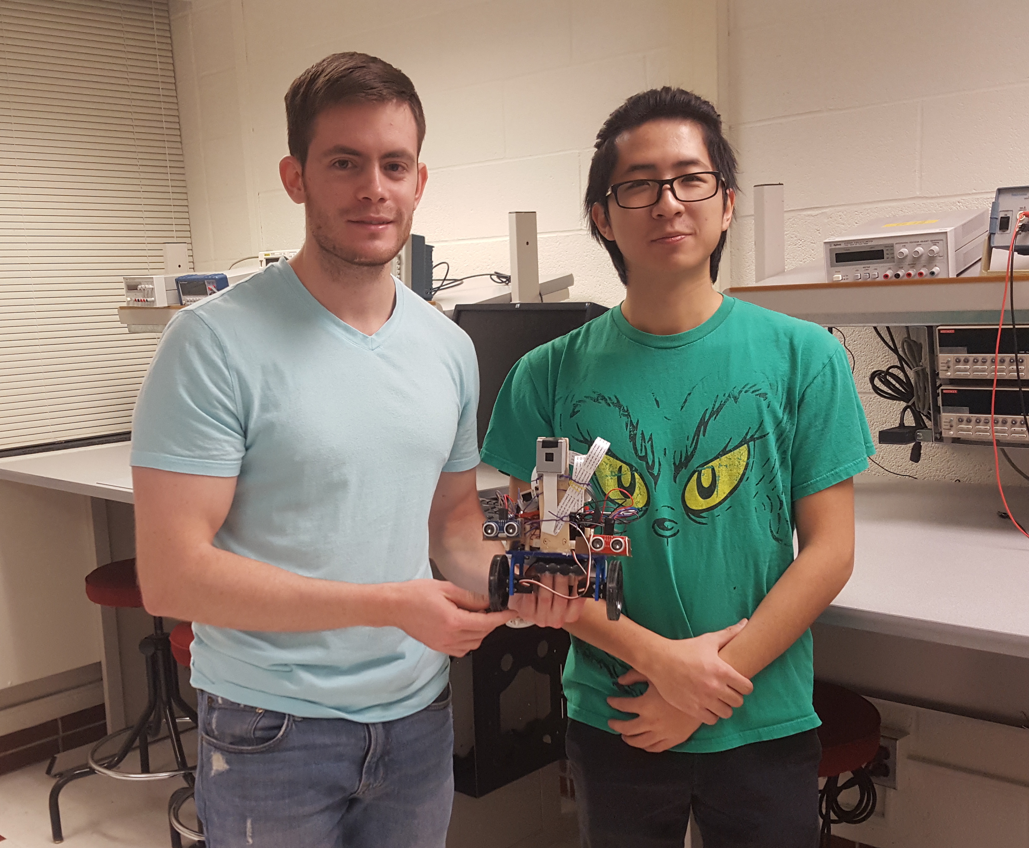
Video: Final product demonstration
Objective top
"An inexpensive and reliable object finding robot with obstacle avoidance capabilities"
As the world of robotics becomes more popular, more people have begun to rely on autonomous systems that do everything for us. We have created a system that is able to search for a user-specified target based on RGB patterns and move towards such object until it is 10 cm away from it. Our robot is also able to avoid all obstacles that it encounters on its way to the target. The system is controlled by a Raspberry Pi unit that takes signals from a Pi-camera and four ultrasonic sensors.

Introduction top
Our system is controlled by a Raspberry Pi 2 unit that takes signals from a Pi-camera and four ultrasonic sensors, two located on the front, and one on each side of the robot. The camera is in charge of looking for the target by actively searching for a pre-specified color, which we have selected to be green (color of the target). Four ultrasonic sensors detect obstacles that are at 10 cm from the robot's sorroundings. When an obstacle is detected the robot takes action according to our algorithm in order to avoid it. Once there is no obstacles in its proximity, the robot continues its course towards the target. Although for the demonstration we chose a small area for the robot to navigate in, as seen in the video above, our product can be navigate in larger setups and successfully find the target. FindBot can also be adapted to find other targets; the only thing the user needs to do is change the RBG pattern to be detected. Our product provides a reliable and inexpensive object finding system for computer vision applications.
Hardware
Our system is composed of a Raspberry Pi 2, a Pi-camera, four ultrasonic sensors (HC-SR04) and two servo motors. There are two sonars on the front, and one on each side of the robot (left and right); they are all in charge of detecting obstacles in the proximity of the robot. The Pi is the brain of the system, as it sends, receives, and processes commands based on our implemented algorithm. Using OpenCV the Pi sends commands to the Pi-camera to search for the specified target. Full-rotation servo motors are fundamental in the motion of the system.
Software
The software implemented was written in Python, and it is based on a polling algorithm that waits for echo pulses from the sensors to take decisions based on sensor readings. The system sends a command to the servo motors to go forward as soon as the camera detects the specified target. The robot will continue to go towards the target as long as it does not detect any obstacles; if it does (within a distance of 10 cm), FindBot turns left or right depending on sensor readings from the side sensors in order to avoid the obstacle. After no object is detected on either side, the robot then turns into the direction it had before detecting the obstacle. Then it searches for the target again, and moves towards it. The Software section below provides more details on the algorithm.
Miscellaneous
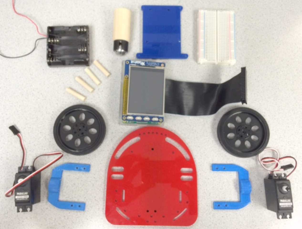
The chassis and wheels used for the project were provided in Lab 3 of the course. The assembly had already been done for that lab, thus we only had to install the sensors and Pi-camera. An external 4.8V battery was purchased in order to power the servo motors. An additional power bank was used to power the Pi.
Design & Testing top
Hardware
Servo Motors
We used Parallax continuous rotation servo motors (datasheet here) to drive the wheels of the robot. Servo motors are ideal for bidirectional continuous rotation and are easy to install/use. Shown below in Figure 1 is the wiring diagram for the servos.
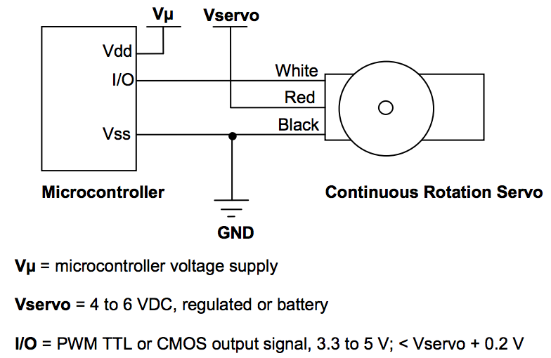
Fig.1 Schematics for Parallax Continuous Servo Motors
As it can be seen in Figure 1 above, a Vdd (red), ground (black) and I/O pin (white) wires are the three connections for the servo. Vdd was provided by an external 4.8V battery pack. Two GPIO pins from the Pi (GPIO 13 and 19) provide the signal connections for the two servos. The motors work with pulse-width modulated signals (PWM) generated by the Raspberry-Pi by selecting the desired frequency, and duty cycle of the signal. Both, the duty of the cycle and frequency can be calculated based on the time in milliseconds that we want to have the signal ON and OFF. The following set of equations in Figure 2 provide information as to how we selected both values.
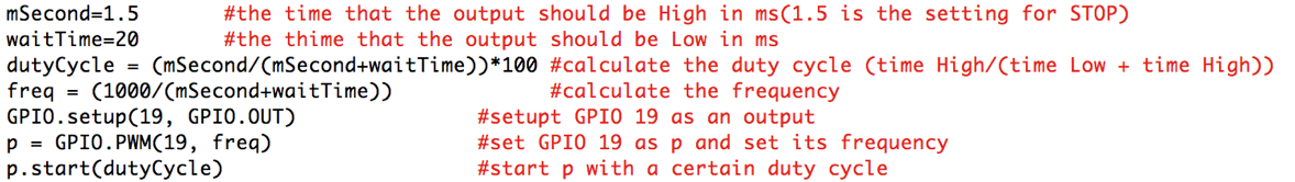
Fig.2 Setting up PWM to drive servo motors
As shown in the figure above, to provide a PWM signal to the motors, the ON and OFF times of the signal need to be specified. Rotational speed and direction are determined by the duration of a high pulse, in the 1.3–1.7 msec range, 1.5msec being the stop condition. To obtain a smooth rotation, the servo needs a 20 msec pause (OFF time) between pulses as seen in Figure 3 below. As shown in Figure 2 above, the duty cycle is calculated from the ON and OFF times, which is simply the ratio of the ON time by the sum of the ON and OFF periods multiplied by 100. Once the duty cycle is known, it is straight forward to obtain the frequency, as shown above. With the duty cycle and frequency the signal can then be sent to the GPIO pin to rotate the motors.
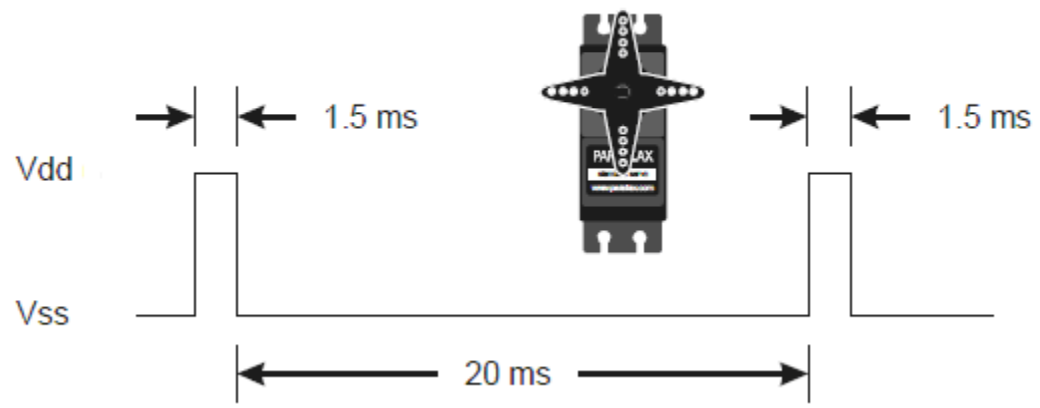
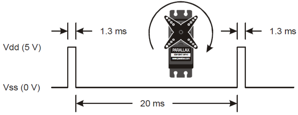
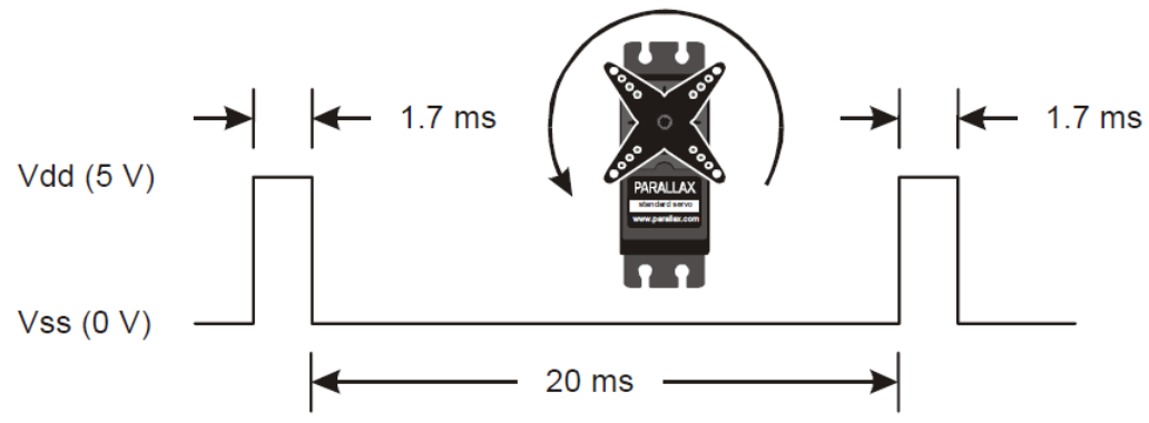
Fig.2 Selecting direction of rotation of the servo motors based on the ON time
As it can be seen, the speed of the motors are controlled via a PWM input signal. For our application we selected 1.4 msec and 1.6 msec as the clockwise and counterclockwise ON times, respectively; that is, the motors do not rotate at full speed. This speed worked very well for our specific application because high speed was not a priority for us. Figure 3 below shows the PWM signal obtained on the oscilloscope for the stop case (1.5 msec ON time).
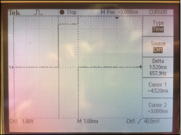
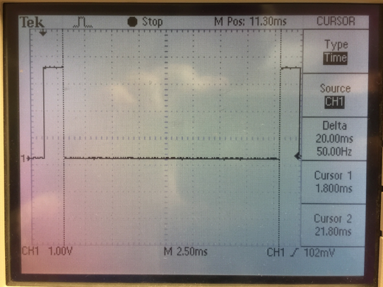
Fig.3 Measured PWM signal for the stop case -- 1.5 msec ON time (left) and 20 msec OFF time (right)
Ultrasonic Sensors
As mentioned above, four ultrasonic sensors were used in our system. Two sensors were place on the front, one on the right and one on the left side of the robot. The ultrasonic ranging module is the HC-SR04, which provides 2-400cm non-contact measurement function, with a ranging resolution of 3mm. Each module, which we purchased from RobotShop, includes an ultrasonic transmitter, receiver and control circuit. The operation of the sonar is initiated by supplying a short pulse of at least 10 μsec to the trigger input. Then the module sends out an 8-cycle burst at 40kHz, after which an echo pulse is raised. The echo pulse is then reset after the ultrasound has bounced off of the object and reached the receiver side of the module. Thus, the echo pulse is proportional to the distance between the sensor and the object; the pulse increases as the distance gets larger. Calculating the time the echo pulse remains HIGH provides information about the distance of the object from the sensor. Figure 4 below shows the timing diagram of the sonar module.
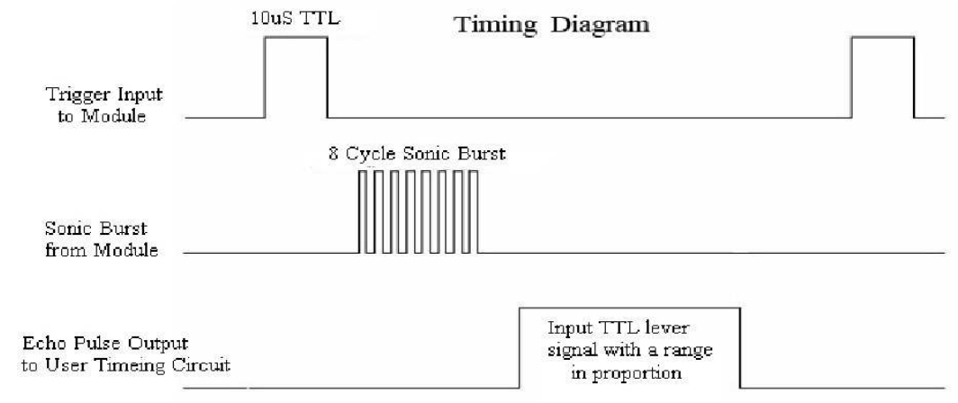
Fig.4 Timing diagram for ultrasonic sensor HC-SR04
Calculating Distances with Sonars
By measuring the time the echo signal remains HIGH we can calculate how far the object/obstacle is from the sensor. Since the speed of sound is 340 m/s, the distance is obtained by: d=t_H*v_sound/2 =t_H*(340m/s)/2. It is recommended by the manufacturer to wait at least 60 msec between triggering events in order to prevent signal interference. Shown below in Figure 5 are the waveforms for the trigger and echo signals of an object located very far (left image) and 10 cm (right image) from the sensor.
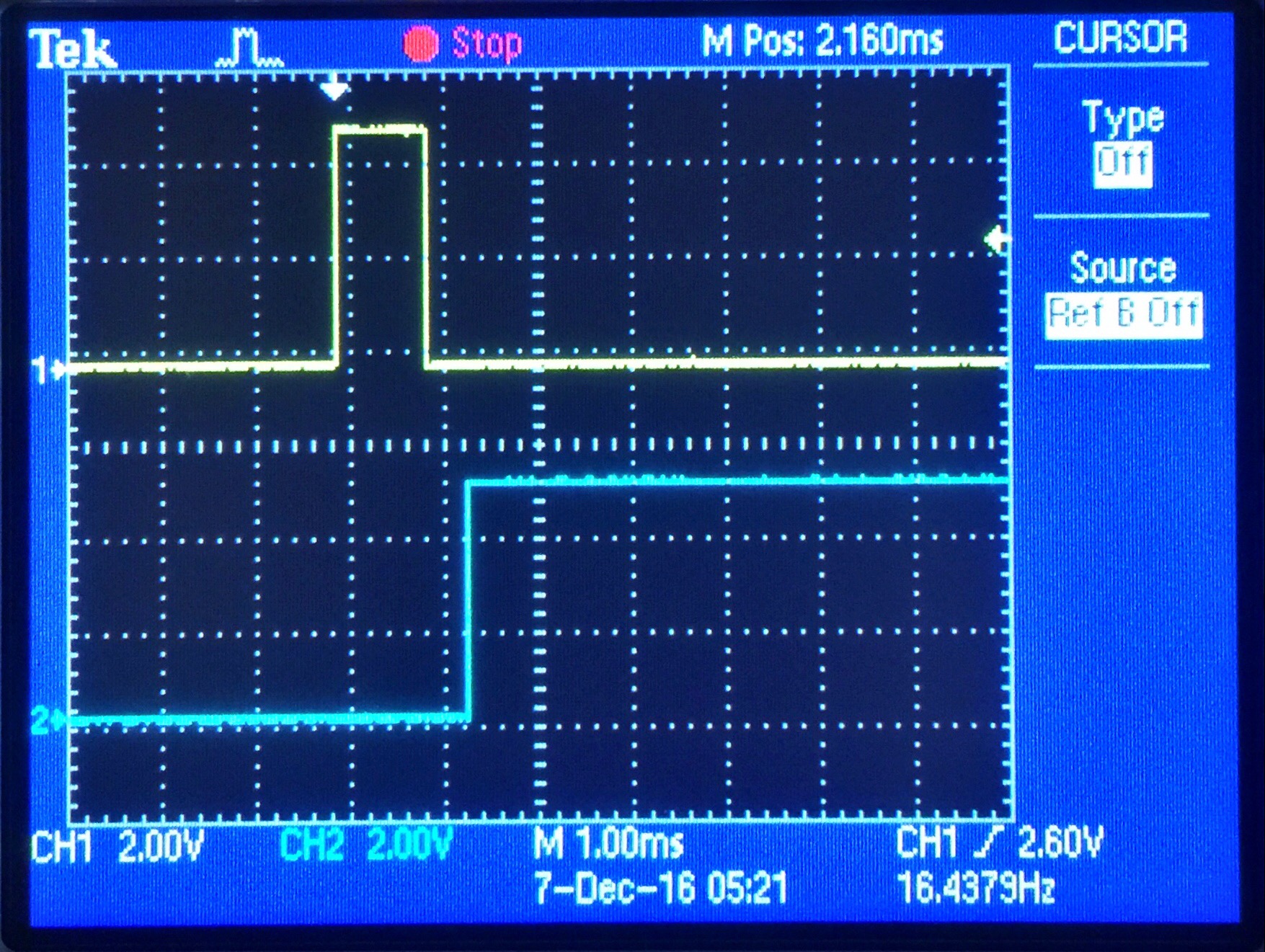
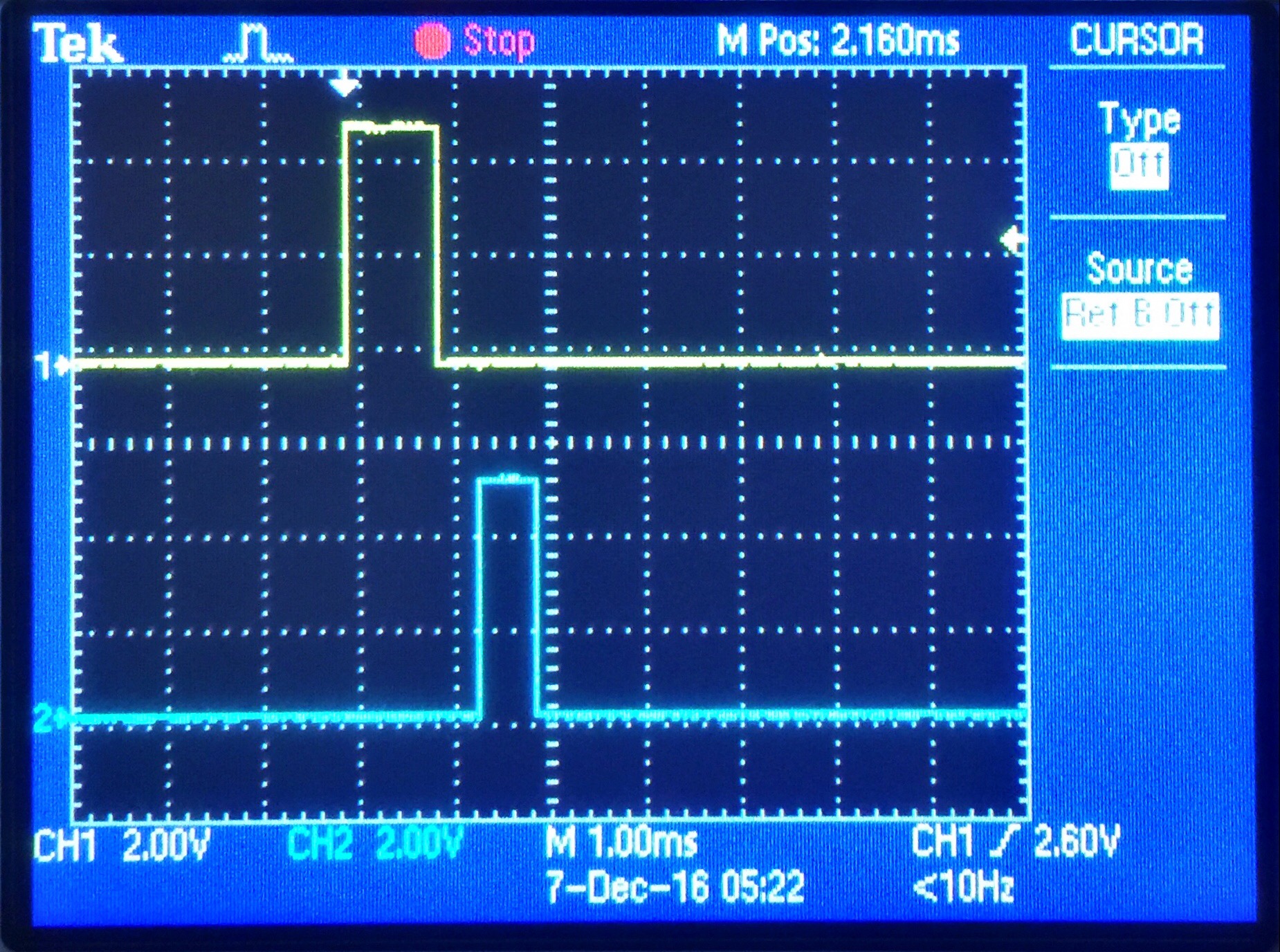
Fig.5 Trigger (yellow) and echo (blue) signals taken from an HC-SR04 ultrasonic sensor at different positions from an obstacle. Left image depicts an object positioned very far from the sensor; right image represents the echo pulse for an object located 10cm away from the sonar. Notice that the trigger pulse is the same for both, which is what we want
Echo Pulse Detection
As mentioned earlier and depicted in Figure 5 above, after the trigger pulse is set and the internal 8-cycle burst is emitted, an echo pulse is set HIGH. The pulse then resets after the signal bounces off of the obstacle and reaches the receiver side of the sonar. In order to compute the distance of the object from the sonar, it is important that we accurately measure the length of the echo pulses for each sonar. To do this, we detect the moment at which the echo pulse goes HIGH, and wait until it goes back to LOW; then we compute the time for which pulse was HIGH, which allows us to calculate the distance of the obstacle from the sonar.
It is
important to note that a single trigger was set for all sensors using GPIO pin 21, and was defined as an output pin. GPIOs 27, 5, 16 and 17 were set as input pins for the echo pulses of the right front, left front, right and left sensors, respectively. Figure 8 below illustrates the schematics of our system.
Trigger Pin of the Sonars
The HC-SR04 sonar modules have 4 pins: Vcc, GND, Trigger and Echo. The operating voltage is 5V, which is supplied by a battery pack. The working current is 15 mA. The trigger and echo signals are 5V pulse. To reduce the amount of GPIO pins used, we decided to drive the four sensors with the same trigger. Since the output of the GPIO pins are 5V, it was not necessary to use a level shifter or boost converter to drive the trigger pin; thus, the GPIO pin on the Pi directly feeds the trigger inputs on the sonar modules, as shown in Figure 8 below. This, on the other hand, raised questions about possible interference between sensors and capability of a single pin to provide a working current to the sonars. However, after some testing we were able to see that triggering the four sensors with the same trigger does not introduce inaccurate measurements.
Voltage Dividers for Echo Signals
It was necessary to build four voltage dividers to reduce the 5V echo pulses from each sonar to 3.3V, which need to be captured by the Raspberry Pi defined-input pins. This was necessary because GPIO pins can only handle a voltage of 3.3V. For this we selected 1kΩ and 2kΩ resistors, and built four voltage dividers, as shown in Figure 7 above.
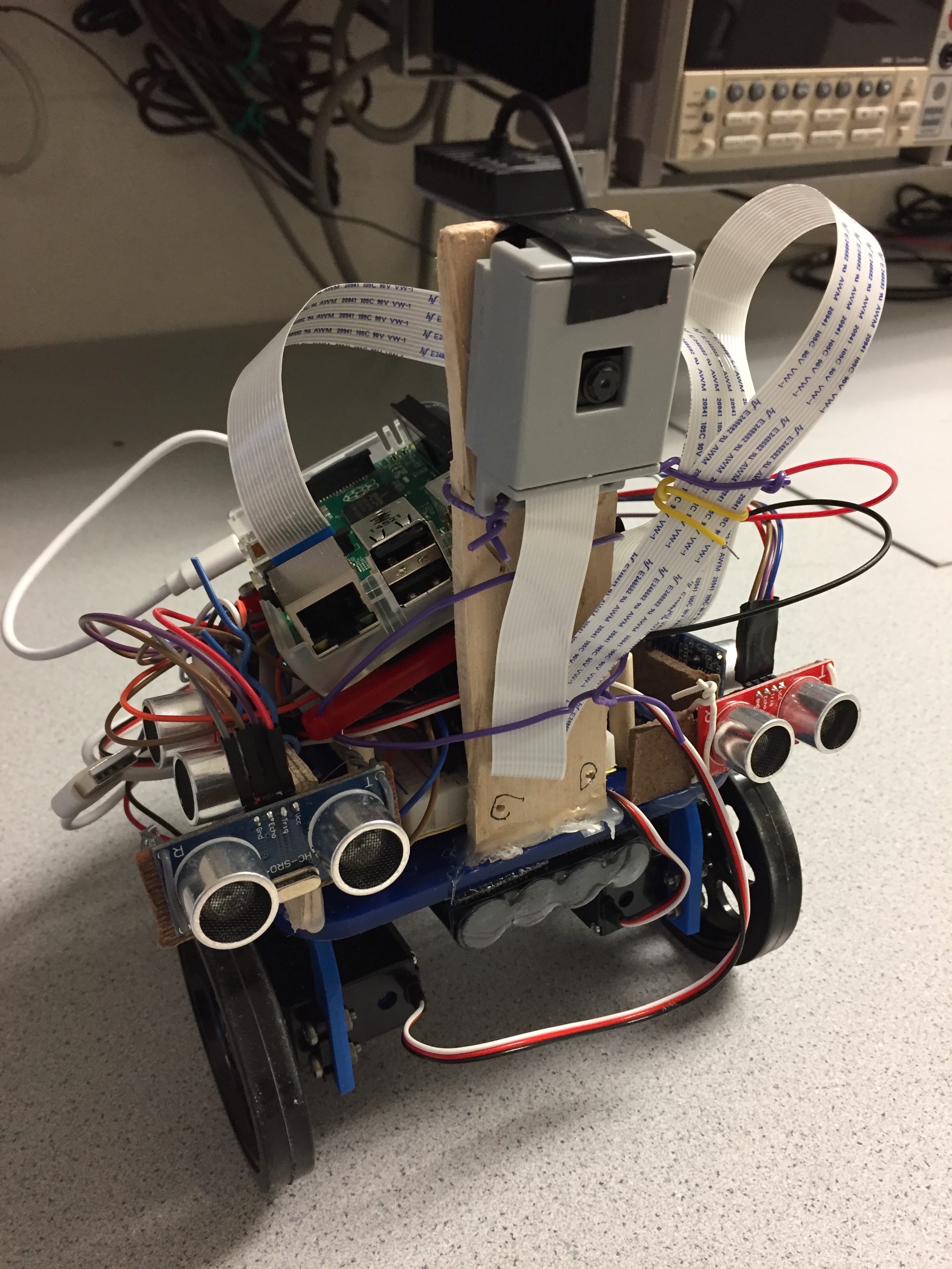
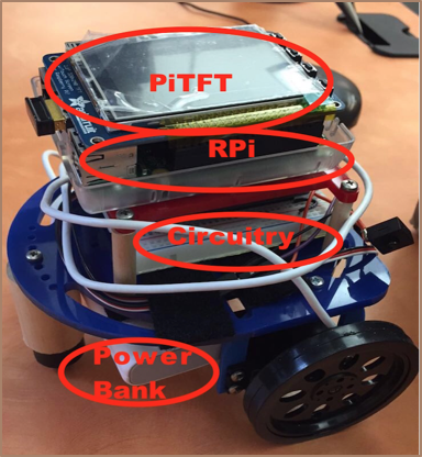
Shown below in Figure 7 is the final product of our system after the Raspberry-Pi, sensors, servos, Pi-Camera and battery pack have been placed on the chassis.
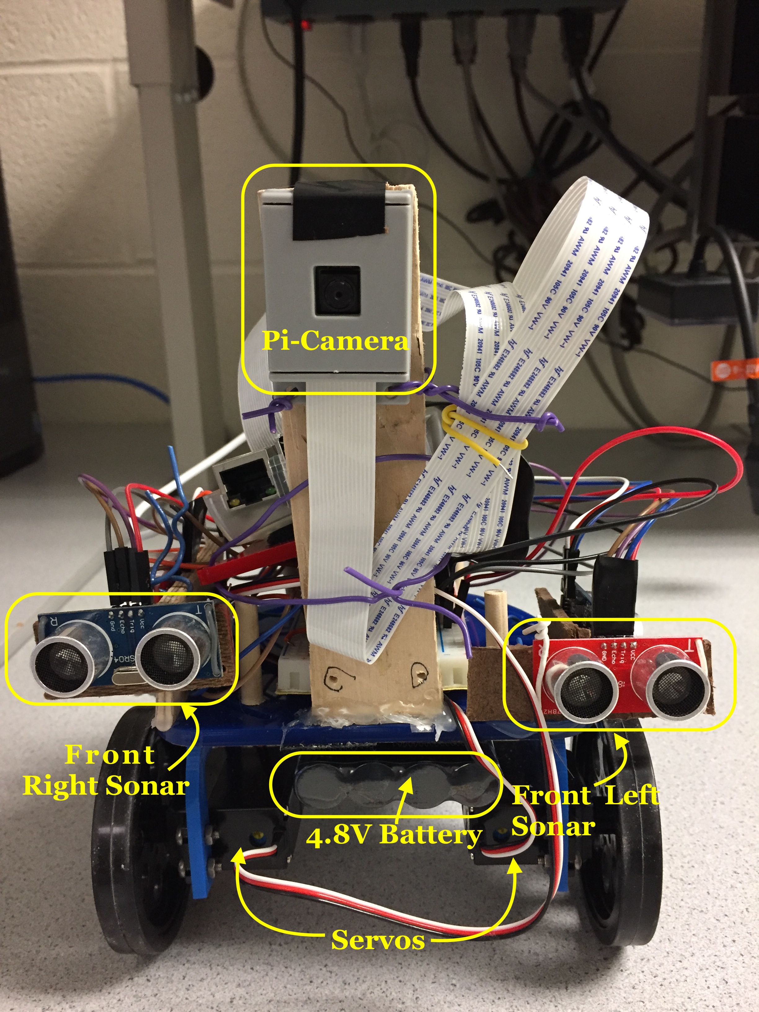
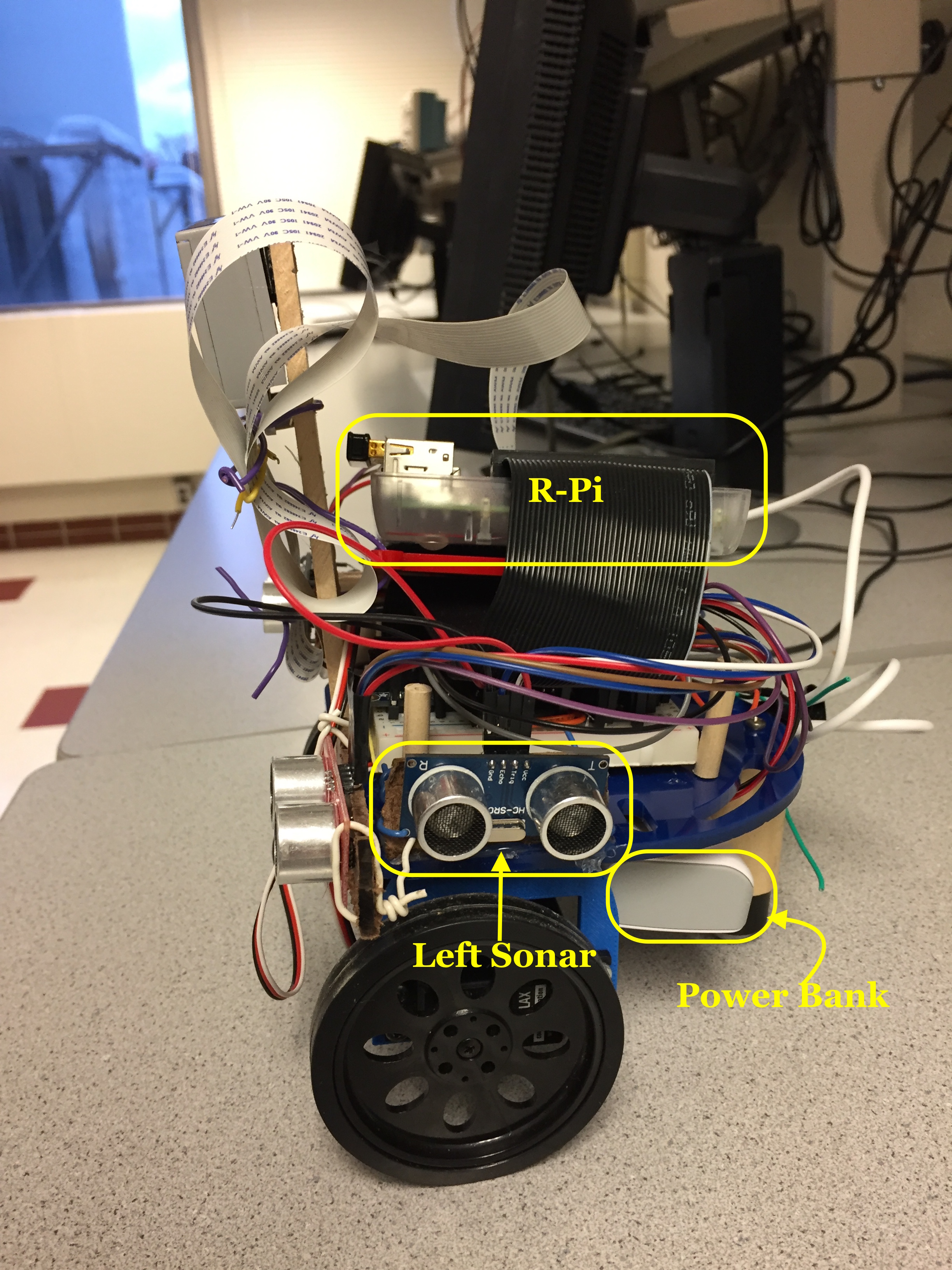
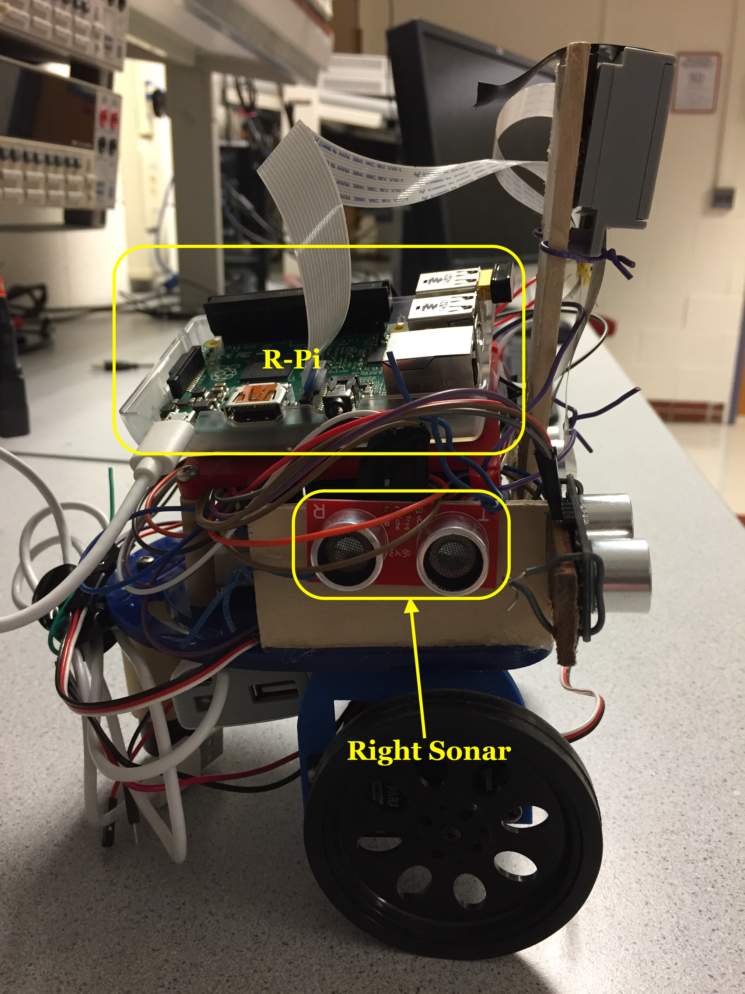
Fig.7 Final robot setup. All components installed on the chassis of the robot
System Design & Schematic
Shown in Figure 8 below illustrates the complete schematic of our system.
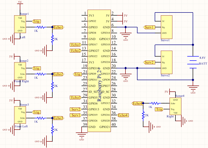
Fig.8 Complete system schematics
Software top
Software Development
The software for our system consists of two major functions/algorithms: a. Target Finding via OpenCV and b. Obstacle Avoidance Algorithm. The developed algorithms are discribed as follows:
1. Target Finding via OpenCV
The main component of our robot is to be able to recognize a user-specified RGB color pattern. We have selected the color green as the color to be recognized, since it is was not a common color in the testing environment/lab. We did this in order to avoid detecting random objects. To perform the pattern recognition, as mentioned earlier, we used a Pi-Camera that continuously searches for the target. In order to set up the camera, OpenCV library needed to be downloaded and installed on the R-Pi. OpenCV is an open source computer vision and machine learning library. The steps we followed to download and install the software are as follows and available here:
a. Update and upgrade Raspberry Pi and existing packages. This includes downloading and installing some image I/O packages that allow to load various image file formats from disk
b. Download OpenCV source code
c.
Install and compile OpenCV source code (we installed OpenCV 2 on first attempt, then we had to install version 3 due to some difficulties). Installation steps are different for Python 2.7 and 3.
d. Test software
We had several issues completing this process. In our first attempt to get OpenCV set up, we installed OpenCV version 2 because the SD card was running low on free space. After about 20 hours for the setup and some tests we ran, we found that the OpenCV was not working properly. The speed on the Pi reduced and the software was extremely low and inoperable. We even got segmentation faults every time we ran our code. Therefore, we decided to use a larger SD card (16GB) and try a later version of OpenCV (version 3). After some hours we got the software to work. The speed improved but was not optimal. There was evident lagging in the software. However, given that our application is not speed dependent, we decided to proceed with the other tasks. We think that either the version of the Pi (we're using R-Pi 2+) or the Python version might be responsible for the low speed of the software.
The next step was to become familiar with OpenCV, specifically learn how to recognize objects. After some research and tests, we were able to successfully program our system so as to recognize the color green.
As mentioned earlier, the detection of the green color was based on the RGB pattern, which was set/selected in our Python program. The robot continuously checks for such pattern and moves towards it as soon as it detects it (and there are no obstacles in front of it).
It is important to mention that the distance of the target from the object is defined by the radius of the green pixels detected by the camera. For our application, a radius greater than 3 indicates that the robot has yet to arrive to the target. When the radius is equal to 3, the robot rotates 360 degrees indicating that the target has been successfully found.
In addition, in order to keep track of the target, the x-coordinate is always recorded. This allows the robot to rotate and align itself with the target in cases it deviates from it. It was not necessary to keep track of the y-position of the target because it is always fixed at a given position. However, if we wanted to add more complexity in the system by working with a moving target, this condition has to be changed.
Figure 9 below shows the software setup for the PiCamera module and other features, as well as the libraries that were included in the project.
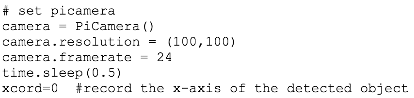
Fig.9 Libraries for computer vision used (lef t) and setup of PiCamera (right)
1. Obstacle Avoidance Algorithm
As mentioned earlier, four ultrasonic sensors are in charge of avoiding collisions of the robot with obstacles as it navigates towards the target. Our first design involved only two sensors, one on the front and one on the left side of the robot, as seen in Figure 10 (left) below. With two sensors, the robot only turns left if it meets an obstacle. With this approach, the robot was able to solve only certain cases, and experienced collisions during its course to the target. Then we tried using three sensors to improve the system's navigation through the "maze," as shown in Figure 10 (left) below. With three sensors, FindBot turns left or right based on the feedbacks from the sensors on the two sides. If the left side sensor has a small value reading, that means there may be an obstacle on the left side, so it will turn right to avoid that potential obstacle. The opposite procedure is done when an obstacle is detected on the right side of the robot. However, as we encountered in our many testings, there were cases where the robot was not able to see objects located at positions greater than the focal angle of the front sensor. This is illustrated in Figure 10 (right) below. This was because the front sensor was placed right in the middle point of the robot. In order to fix this issue, we decided to include one more sensor in the front of the robot, as shown in Figure 10 (left) below. As it can be seen, the two front sensors were placed on each end of the front side of the robot. This provided a perfect solution to our previous problem. With four sensors, FindBot navigates very well through the "maze" in search of the target!
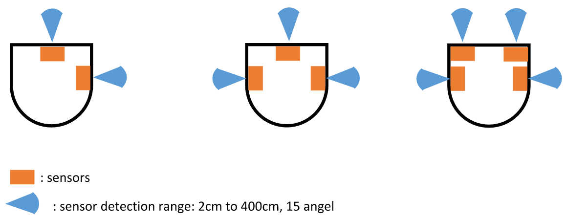
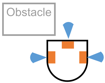
Fig.10 Design process of the navigation algorithm based on sensors used.
The initial instruction by the user to start the navigation of the robot is done wirelessly via ssh. When the robot is given the command to start the navigation, it rotates while it captures frames using the camera. When the system detects the target, the robot moves towards it while also looking after obstacles. When an obstacle is detected in front of it, the robot then processes the information given by the side sensors and takes action accordingly. If a turn is required, the system stores the x-coordinate of the last recorded value of the target. This is done so that, when the robot is done navigating away from the obstacle by moving left or right (and it doesn't detect anything on its sides), it can adjust itself to that given x-coordinate. That is, instead of doing another full rotation in search for the target, the robot rotates towards the last x-coordinate value recorded right before deviating from the target. This approach saves a lot of time in the navigation. It is important to mention that when the robot takes a left/right right turn because of an obstacle, it will continue in that direction (left/right) until it does not detect the obstacle on its right/left sensor. Also, in order to make sure that the obstacle is completely out of the range of the robot we give an extra push right after the side sensors don't detect the presence of an obstacle; this way the robot is free to move without hiting such obstacle. After this maneuver, the robot then searches for the target once again by rotating towards the value of the last recorded x-coordinate of the target. Figure 11 below summarizes the navigation algorithm developed for our application. Figure 12 illustrates the execution of the algorithm in the testing environment.
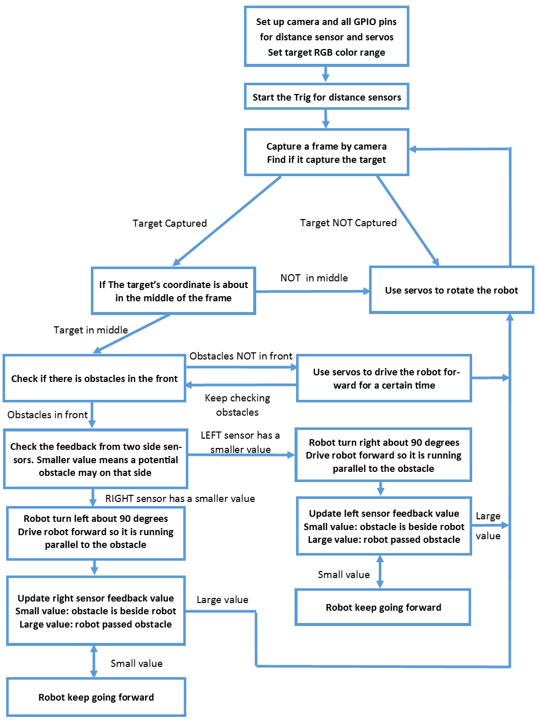
Fig.11 Flow diagram of the navigation algorithm, including target detection and obstacle avoidance
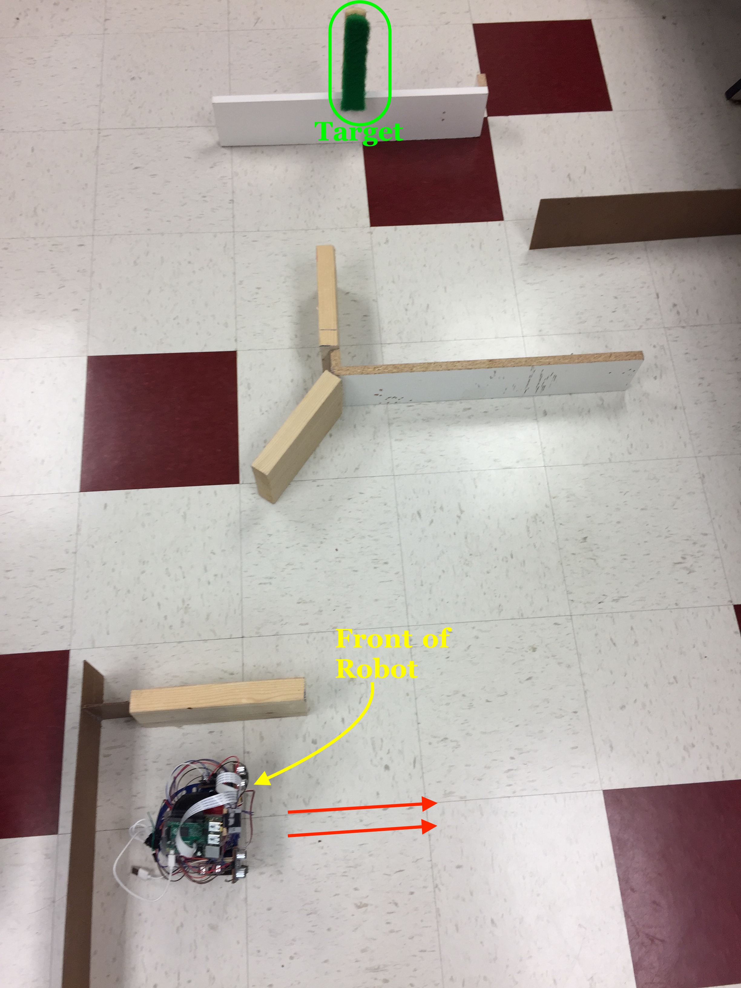
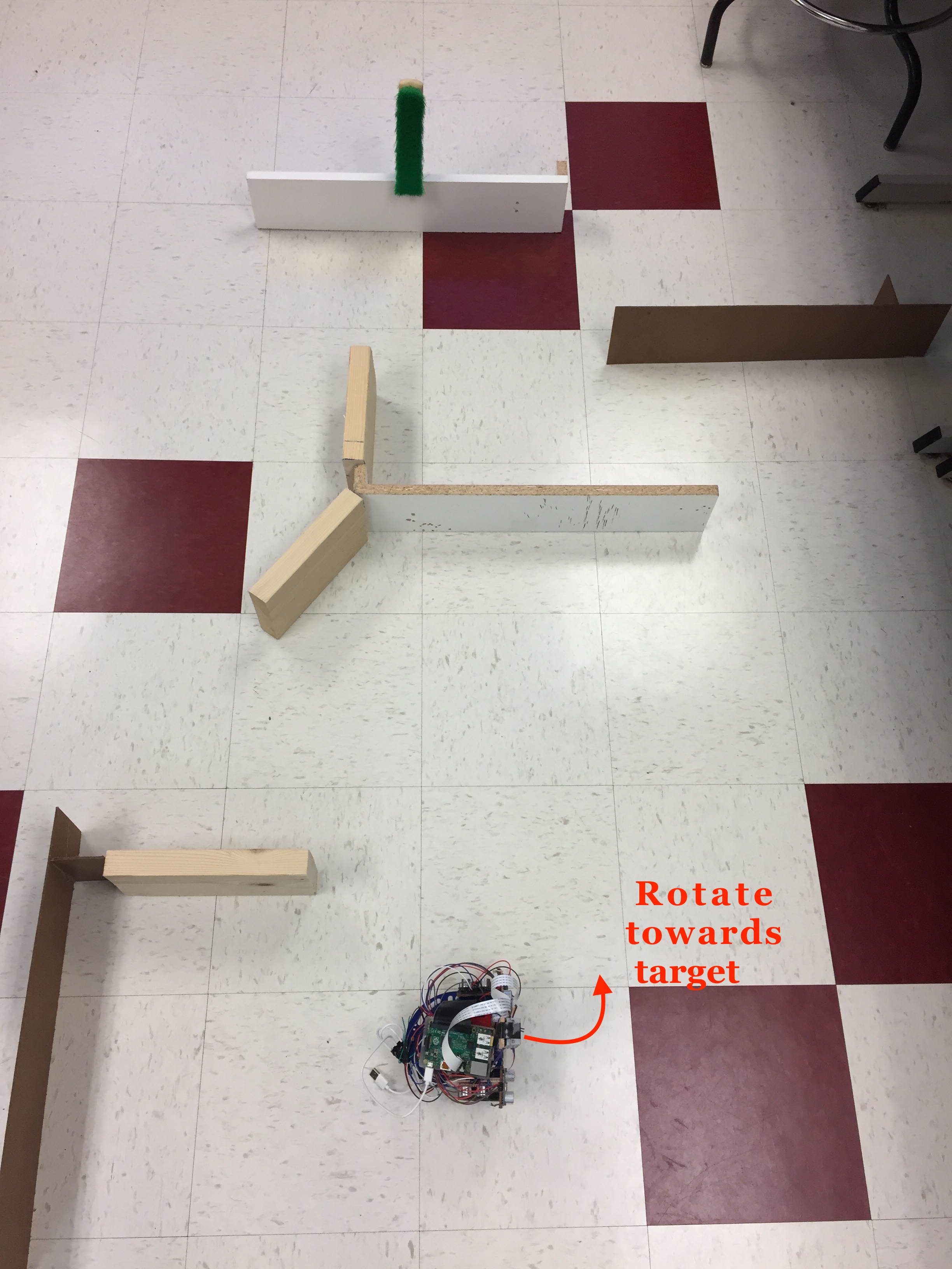
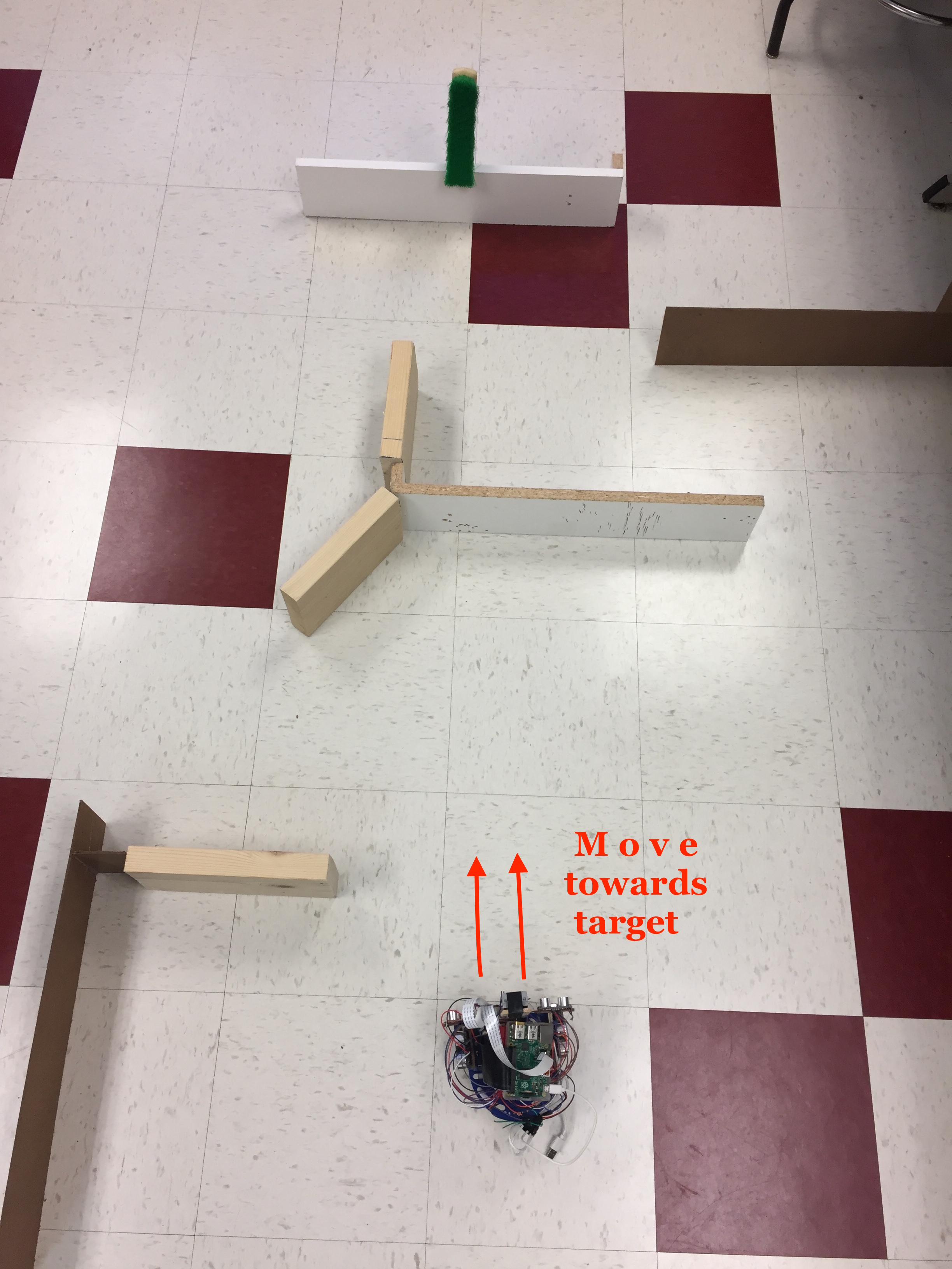
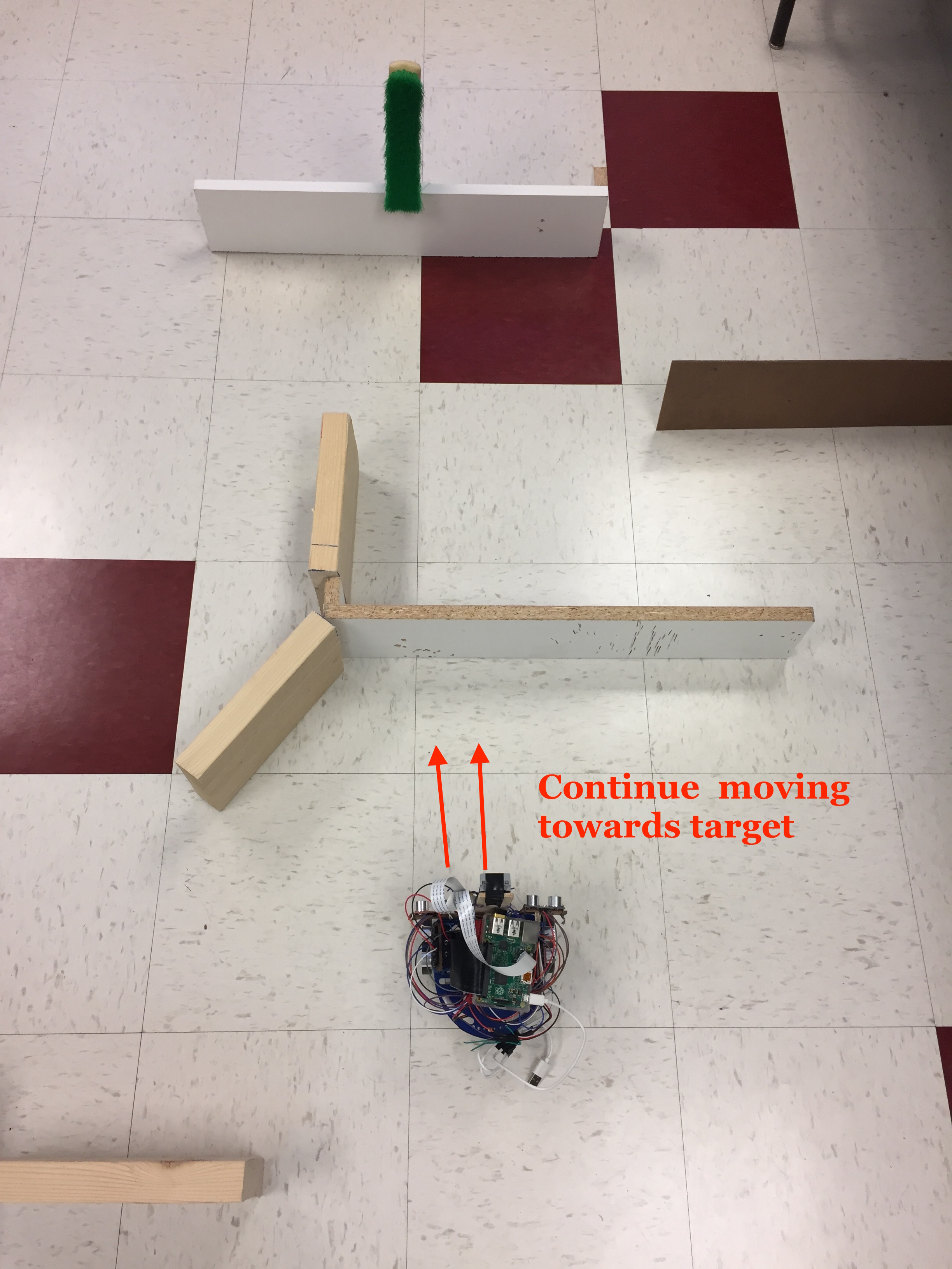
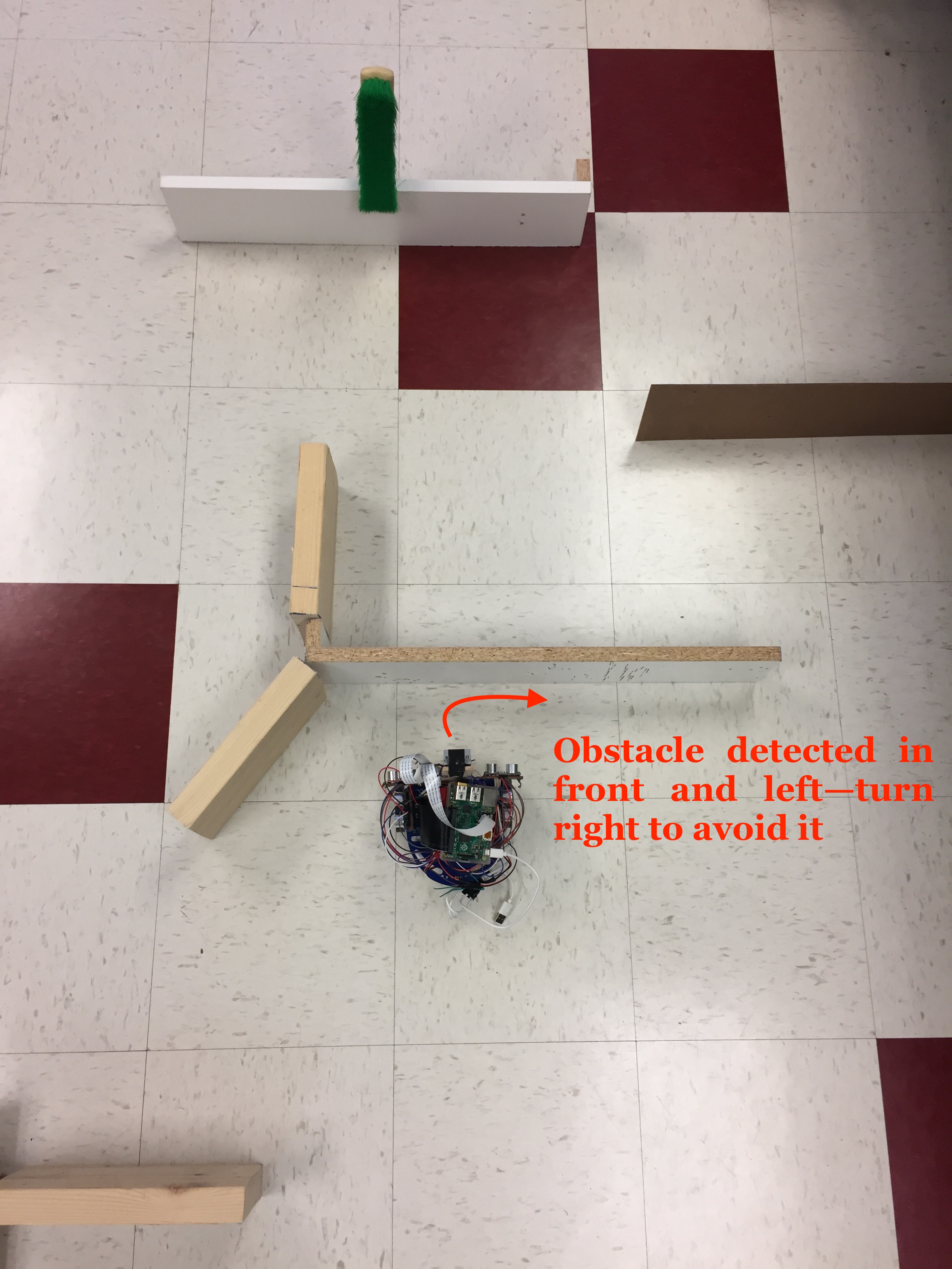
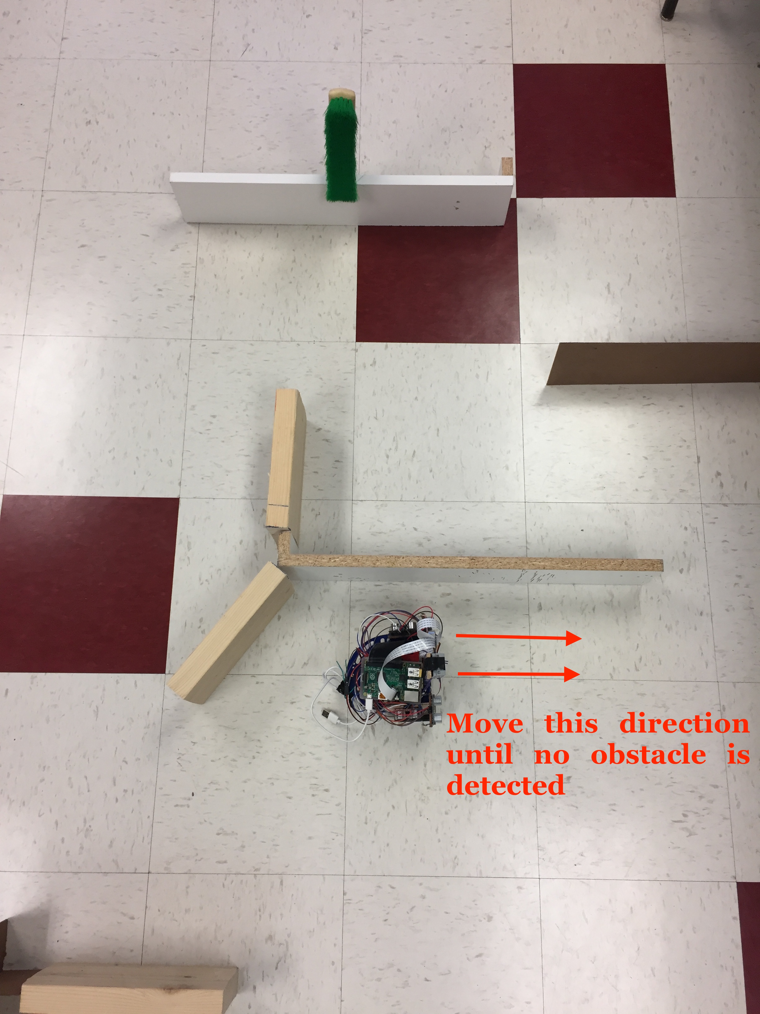
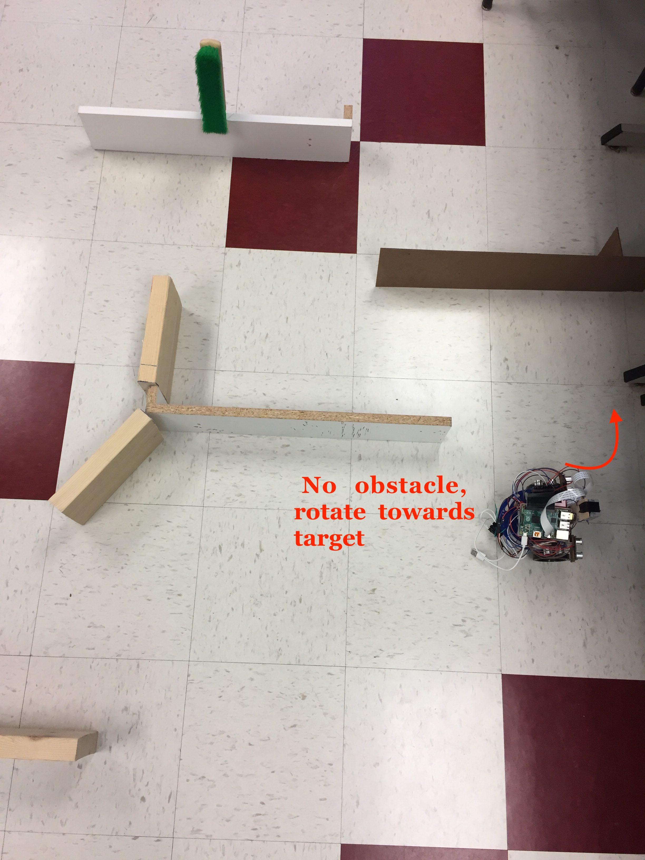
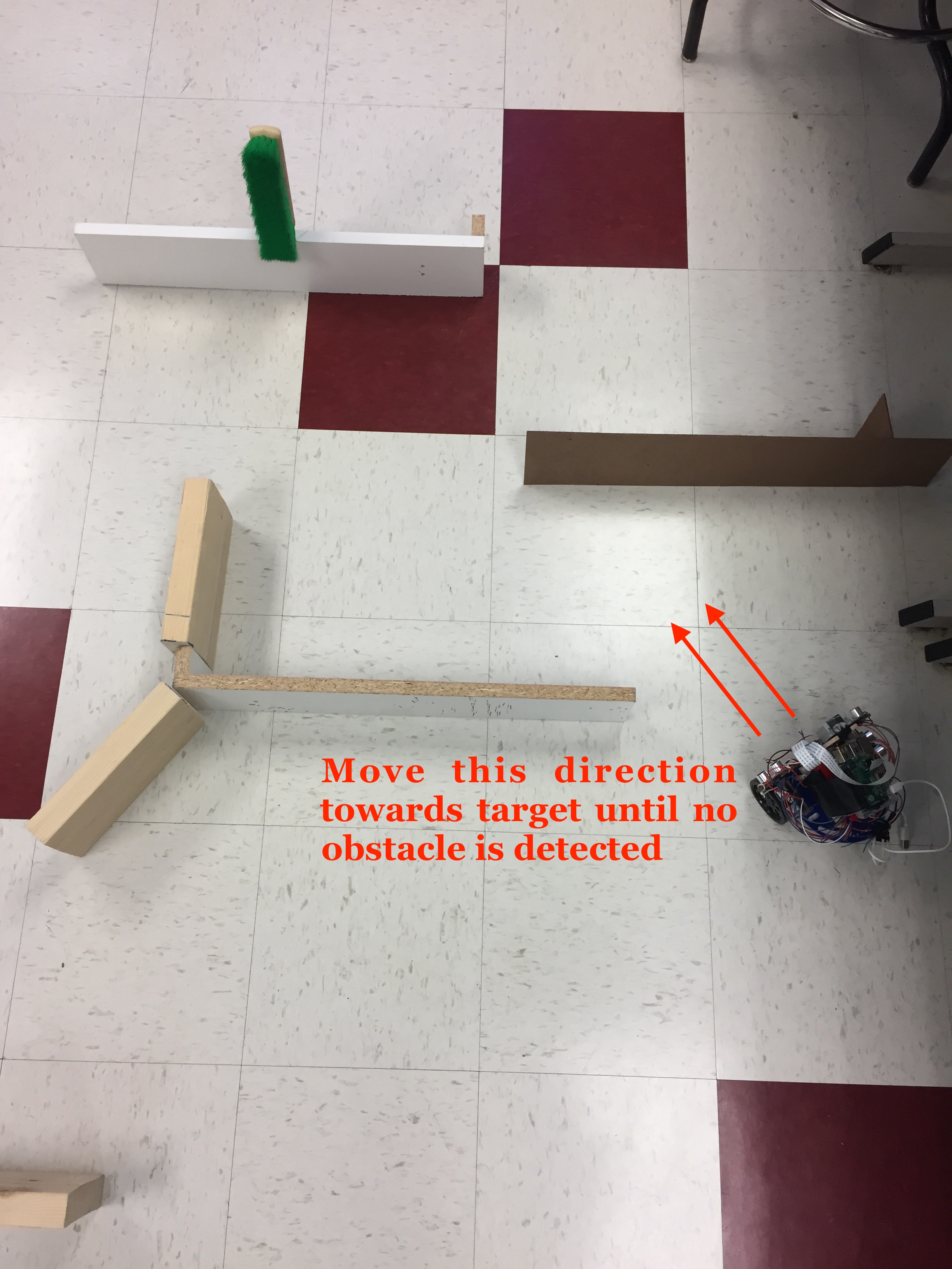
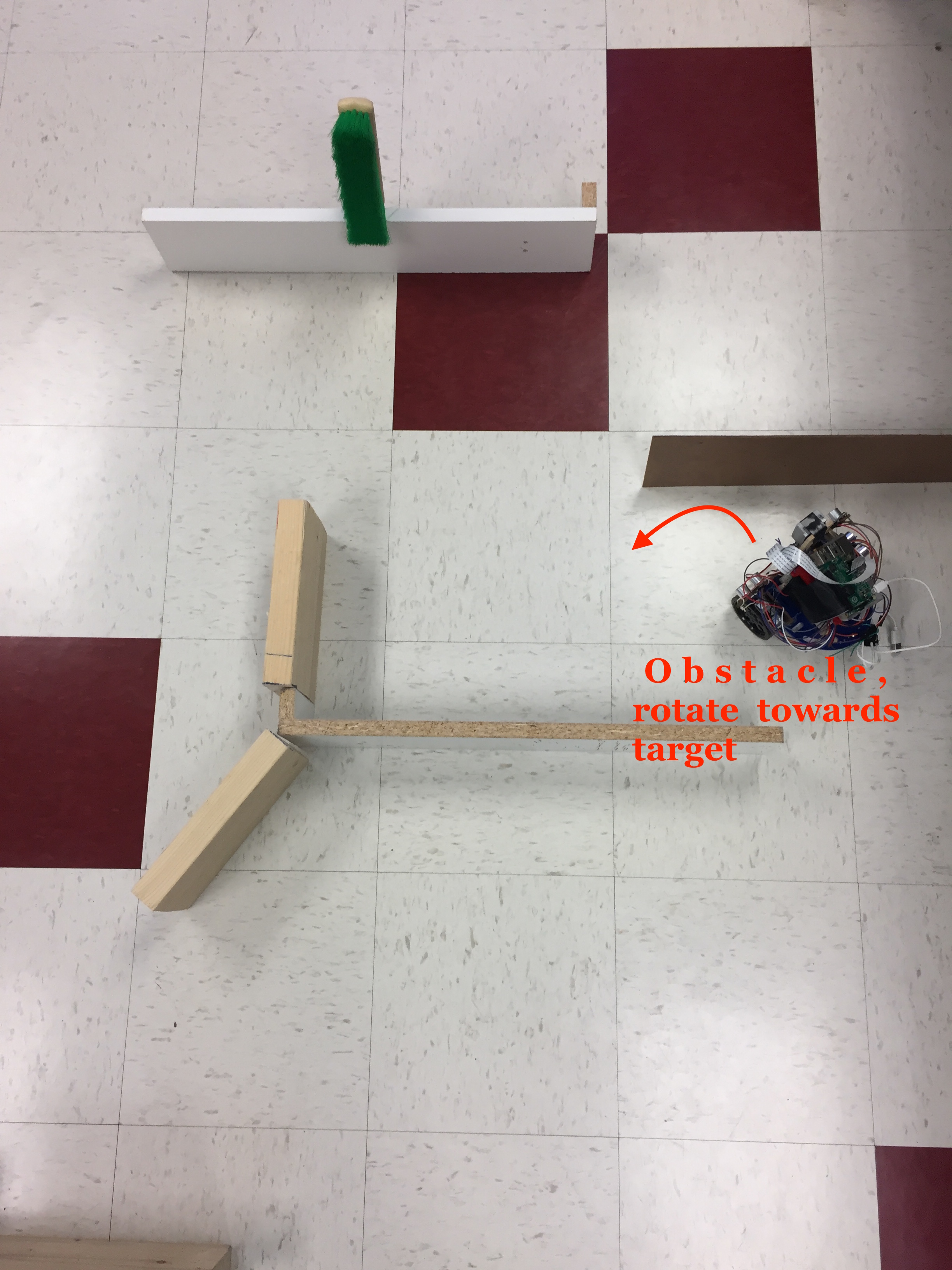
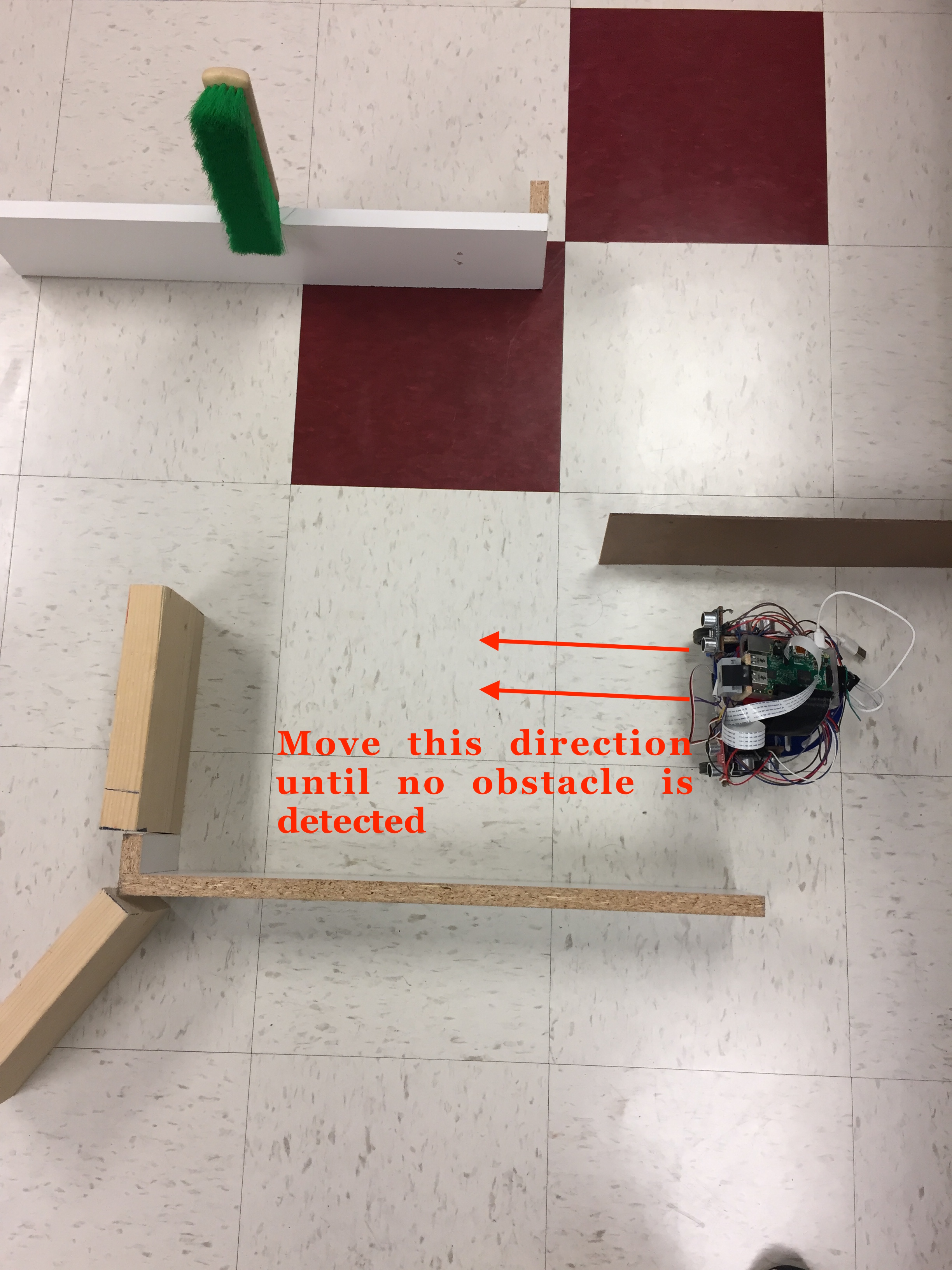
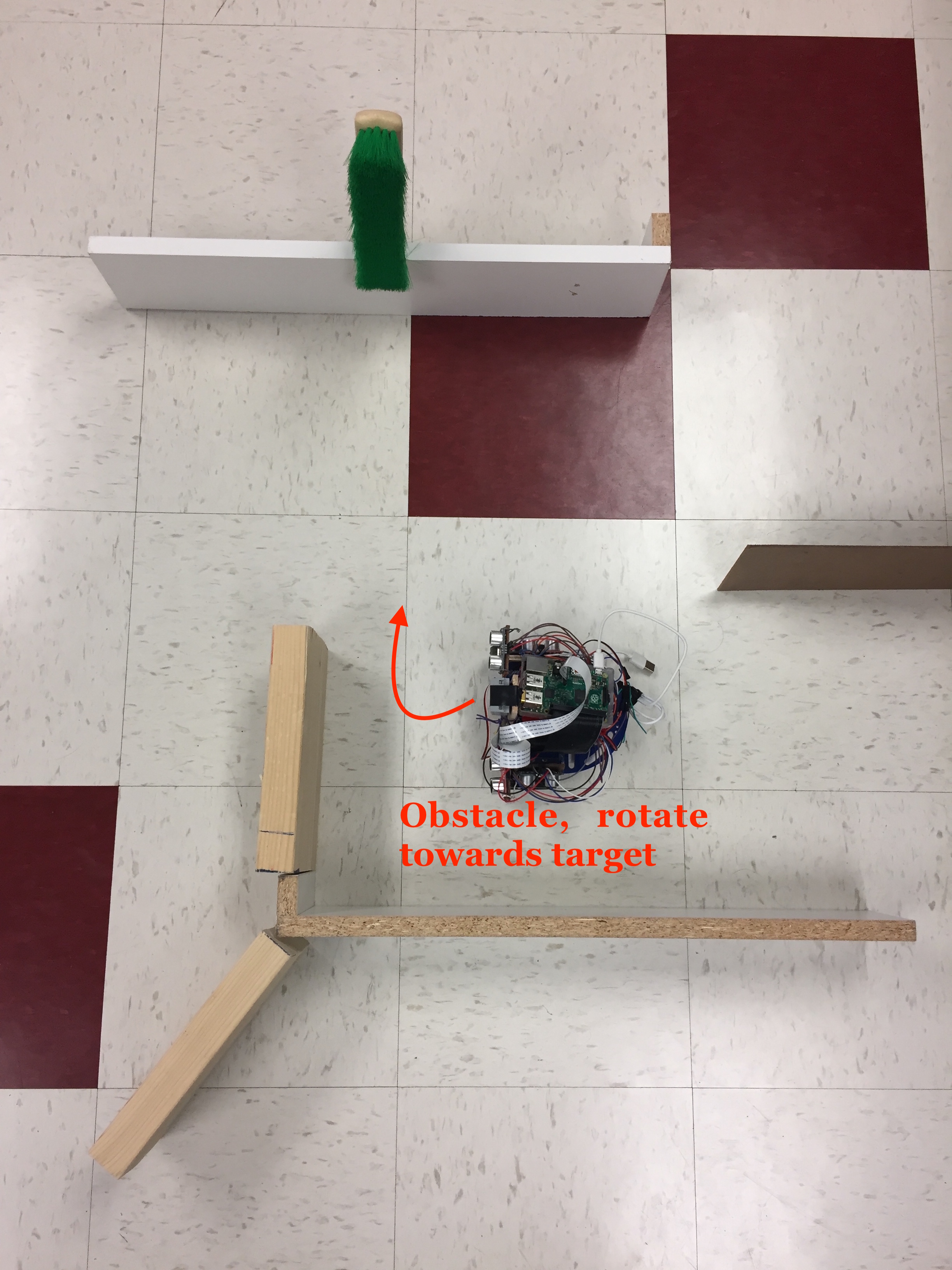
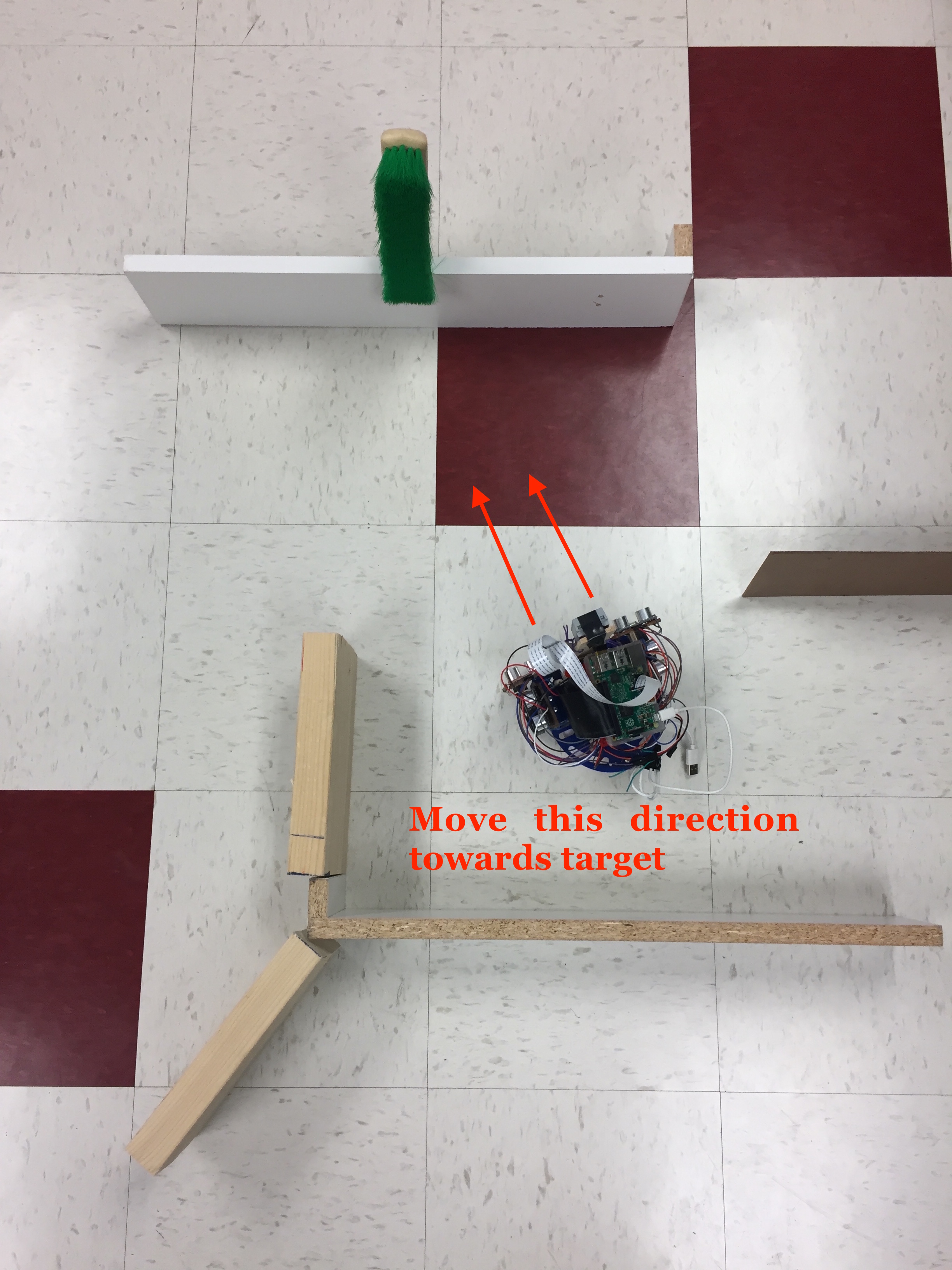
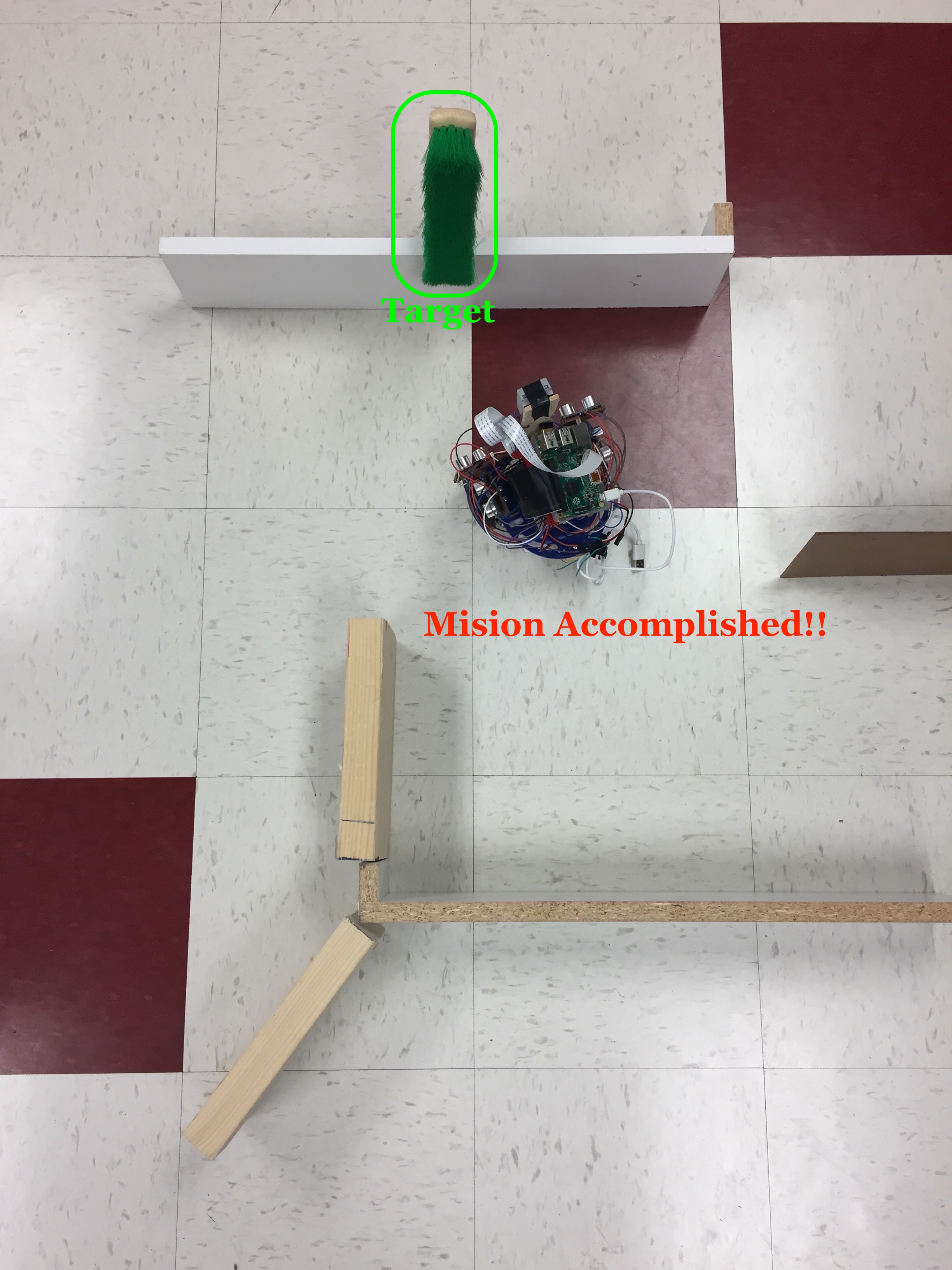
Fig.12 Execution of the navigation algorithm in the testing environment. FindBot doing its thing!
Figure 12 above illustrates the performance of our system as it navigates through the maze. Even though the setup shown in the figure is different from the one presented in the video shown above, FindBot was able to perform equally well. In fact, we tested the navigation in a few other different setups, all of which were successful and accurate. This proves that our algorithm can accurately work in any environment as long as the target is at an appropriate height for the robot to be able to see.
Results top
Accuracy
Our final product is capable of accurately traversing through the "maze" and successfully finding the target. The navigation algorithm provides a robust way for the robot to avoid all obstacles it encounters throughout its course without losing track of the target. The system stores the last x-coordinate value of the target before turning left or right due to a detection of an obstacle. This allows the robot to later continue its navigation in the same direction it had before it encountered the obstacle, without the need of doing a full rotation to search for the target again. This approach saves a lot of time and computation. Certainly, the system works as planned and designed, as we have shown in Figure 12 and in the demonstration video above. Through testings, we have been able to see that the robot is able to avoid all obstacles, as long as the obstacle covers the entire sensor module for the front sensors. There have been cases where the receiver side of a sensor is blocked by an obstacle but the transmitter side is not. This in turn introduces a source of error, in which the receiver is not able to receive the corrent signal. This is mainly because of the small angle of emission and also reception of the transmitter and receiver modules (this angle is 15 degrees as per the datasheet). To solve this issue, better ultrasonic sensors (with bigger working angle) could be used. However, this issue was not a concern in our project, given that it seldom occurs.
Issues Faced
As explained previously, the major issue we faced was with the OpenCV installation. Our first attempt, which was OpenCV2 did not work for our application, as it was extremely slow. Then, with OpenCV3 we obtained a better working software, though still slow. However, because we did not need live video and our application did not require fast data, we were able to work around this issue. We decided to use this installation; luckily it worked for our specific application.
Another problem we had was with segmentation fault messages that we were getting, especially after running our program for a couple of minutes. Specifically, this happened more frequently with our very first approach for measuring the echo signals from the sensors. Rather than using a polling technique, we used callback functions that would detect the falling and rising edge of the echo signal separately. At the beginning, we tried using a sub-function in the program. The sub-function would keep detecting the rising and falling edges from the Echo pin on the sensor, so the program would keep updating the reading from the sensors rather quickly. We used separate pins, one pin for rising edge, and another one for falling edge for each sensor. This way, when the robot is running, it would just take the sensor reading value immediately, and the most updated ones. However, segmentation fault always occured while the program was running. Using only two sensors rather than three or four increases the time span of the program without getting segmentation fault messages. However, after some time running it, we got that error. The segmentation fault occurred rather quickly when using three and four sensors. Because of this, we had to switch to another approach using polling, as we have already explained. When we need the feedback from then sensors, we start to detect the rising and falling edge, and based on the time difference between both events we calculate the distance. This approach fixed the issue with the segmentation fault, even when using four sensors. Our algorithm worked perfectly with this technique.
Despite the issues and limitations we faced, we were able to significantly reduce all sources of possible errors that might have impacted our system. In fact, as it can be seen in the video above, the robot is able to accurately find the target and move towards it, while successfully avoids all obstacles that it encounters in the way.
Thanks to our hard work on this project, we were able to meet the goals outlined in the description presented in our project proposal.
Conclusions & Future Work top
The design and implementation of FindBot: The Object Finding and Obstacle Avoidance Robot was a success. We created an autonomous system that is able to detect a target based on a specified RGB pattern. The system can successfully detect the target (color green) from a distance of up to 4 meters, and move towards it until it is 10cm away. On its way, FindBot accurately avoids all obstacles that it finds by maneuvering around the objects without losing track of the target. In the case where an obstacle causes the robot to deviate from the target, FindBot stores the last x-coordinate value of the position of the target and rotates back towards this position once it has finished avoiding the obstacle. The navigation through the maze is done very smoothly. Ultrasonic sensors are a fundamental part in performing the object avoidance algorithm and keeping the robot from hitting the obstacles it encounters while traversing through the testing environment.
Have we had more time to extend the project, we would certainly have explored adding a Pi-TFT in order to see the live videos from the PiCamera. Then, we would explore creating a website where the user is able to see the recordings live. This would allow the user to keep track of the performance/behavior of the robot. Therefore, the only thing the user would have to do is login on the website, press START to initialize the navigation through ssh, and sit back and watch FindBot do its thing!
Usability
As technology continues to change the way we live and the field of robotics becomes more popular and necessary, more people have begun to rely on automated processes that do our everyday activities. With this project we have created a system that can help in finding a specified target through pattern recognition. FindBot can be used in any environment where an object needs to be found. The only thing the user needs to do is run the program wirelessly via ssh to tell FindBot to look for the target. In addition, our system can be adapted to detect moving targets. This would allow the user, for example, to find his/her pet around the house. FindBot is a very useful product overall, and represents the first steps of even larger systems that can automate and make easier the way we live.
Safety Measures
Our product is very accurate and the sensors dynamically detect any obstacles in its path. Increasing the number of sensors would fool proof our robot from hitting obstacles. But even in its current state, our robot is able to avoid collisions with obstacles with an almost perfect accuracy.
Ultrasonic Sensors
Ultrasonic sensors are fairly resistant to external interference. They are not affected by ambient light or motor noise as there are few natural sources that produce ultrasound. Moreover, the emitters of the sensors are programed to emit pulses which are accurately detected by the intended receiver itself. This also ensures that sensors do not interfere with each other. However, for a larger-scale system it is critical that more sensors be used in order to increase system reliability and performance. In addition, sensors with larger angle of emission and reception would also increase the reliability of the product.
Intellectual Property Considerations
We appreciate the OpenCV installation instructions provided on PyImageSearch by Adrian Rosebrock (link here), as well as his great tutorial on Ball Tracking with OpenCV, from which we learned a lot about the OpenCV features.
We have acknowledged all use of code and have abided by all copyright statements on both code and hardware. We have given credit to all hardware devices that were used in this project, as well as the code that was referenced in our final program.
Appendices top
A. Program Listing
The source file for the project can be seen here. This file is not meant to be distributed and must be referenced when using all or portions of it.
B. Parts List
| Part | Vendor | Cost/Unit | Quantity | Total Cost |
|---|---|---|---|---|
| Raspberry Pi | Lab | $35 | 1 | $35/not included |
| Servor Motors | Lab | $12.95 | 2 | $25.9 |
| Bread Board | Lab | $5 | 1 | $5 |
| Ultrasonic Sensors (HC-SR04) | RobotShop | $2.50 | 4 | $10 |
| Battery Pack | Lab | $5 | 1 | $5 |
| Miscellaneous (wires, resistors) | Lab | $0 | 1 | $0 |
| TOTAL: | $45.9 |
C. Division of Labor
The work done for this project was evenly spread among team members. Both team members contributed in the development of the target finding and obstacle avoidance algorithms implemented in this project. Boling's work on the optimization of the system was fundamental. Alberto's work on the design of this webpage was essential. The contribution of all members was crucial for testing and optimizing the system. The creation of FindBot is a result of the collaboration of both members of the group who spent many hours working on this fascinating project.
References top
This section provides links to external reference documents, code, and websites used throughout the project.
References
Acknowledgements top
We would like to give a special thanks to our professor Joe Skovira for all the recommendations, support and guidance that he provided to us throughout our work on this project. We would like to also thank him for building an amazingly rewarding class from which we learned tremendously. Also, we would like to thank the TAs, especially Jay and Brandom who were our lab TAs, for the continuous support and guidance throughout the semester.